Lighting Overview
Lighting in Computer Graphics is a fascinating and deep topic. To approximate lighting in a digital 3D environment, we have a variety of shading "models". A shading model, or shading algorithm, is just a method used to simulate the appearance of surfaces under light sources. It defines how the color of each pixel on the surface is calculated based on the lighting model (the mathetatical framework that describes how light interacts with surfaces) and the material properties of the surface. It typically takes into account things like the geometry of the surface, the viewer's perspective, and the lighting environment to compute the final color displayed on the screen.
To start off, and before we jump into the code, I'd like to briefly discuss some of the most basic components that our lighting models can made up of, and then give a general overview of some of the most common shading models:
Basic Components of Lighting Models
Components such as ambient, diffuse, specular, emissive, and others are used within lighting models to aproximate how light interacts with objects. These components are the building blocks of a lighting model. In particular, we'll cover these four in code as we discuss and implement 3 of the most basic lighting models later in this chapter.
- Ambient light simulates indirect light that illuminates all objects evenly, regardless of their location and orientation. The ambient light component is crucial in rendering because it simulates indirect light - the light that has bounced off other surfaces in the environment, providing a baseline illumination. This helps to avoid completely dark areas in the rendered scene that would be unrealistic in most real-world scenarios, where light tends to scatter and bounce around. It provides a base level of light so that all objects are minimally visible even if they are not directly lit by a primary light source. It doesn't produce shadows or highlights, and is generally constant and uniform across the entire scene.
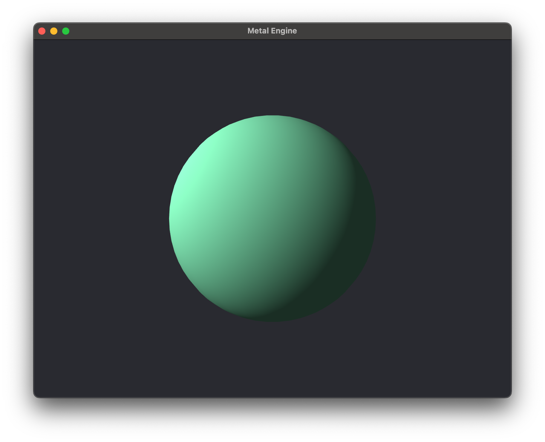
- Diffuse light simulates the light that is scattered in all directions when it hits rough surfaces. It simulates the light that comes from a specific direction, like the sun or a lamp, hits a rough surface, and is reflected equally in all directions. It's used to model the color and intensity of surfaces under direct light without the influence of shiny reflections or glossiness. Dependent on the angle between the light direction and the surface normal.
- Specular light represents the bright, mirror-like reflections that occur on shiny surfaces that are the result of direct reflection, like the glint off of a shiny surface. It's used to simulate the reflective properties of materials and to create highlights that change based on the viewer's perspective. It's dependent upon the viewer's position and the surface's shininess or glossiness, typically using the Phong or Blinn-Phong reflection model.
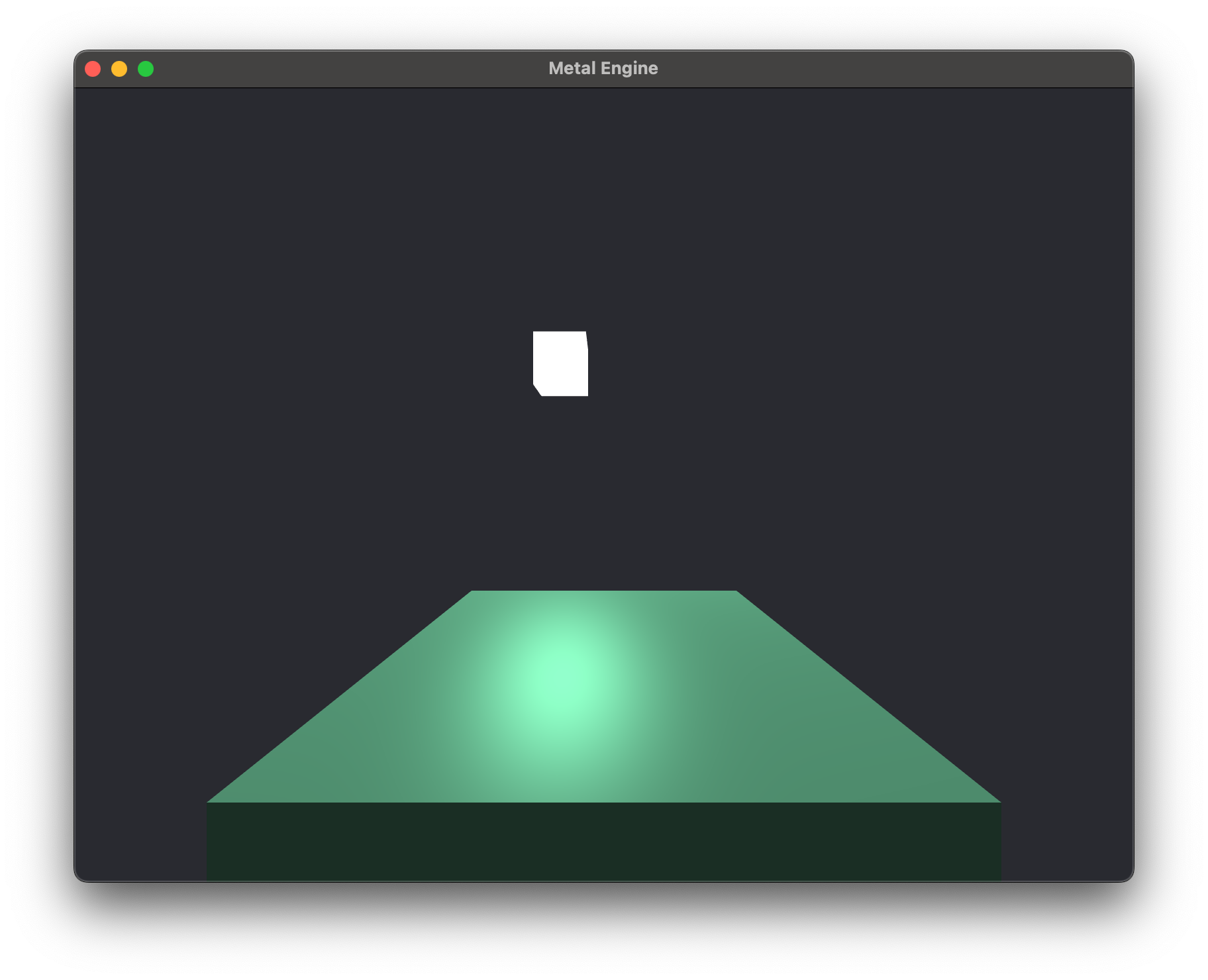
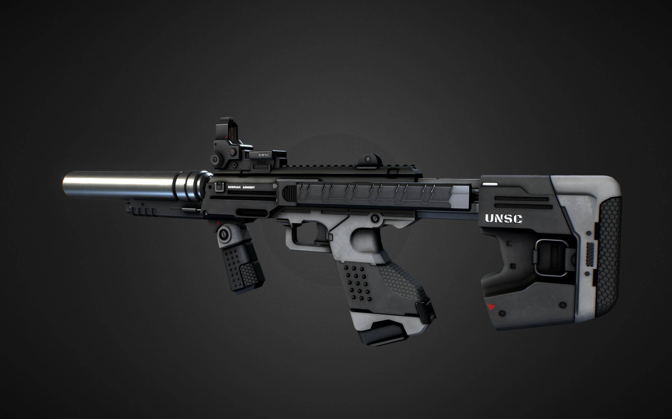
- Emissive light represents objects that emit their own light, like a monitor screen, or a firefly. Its usually implemented through a special "emissive" texture that defines which parts of the model emit light and what color the light should be. It's not affected by other sources of light or the viewer's perspective.
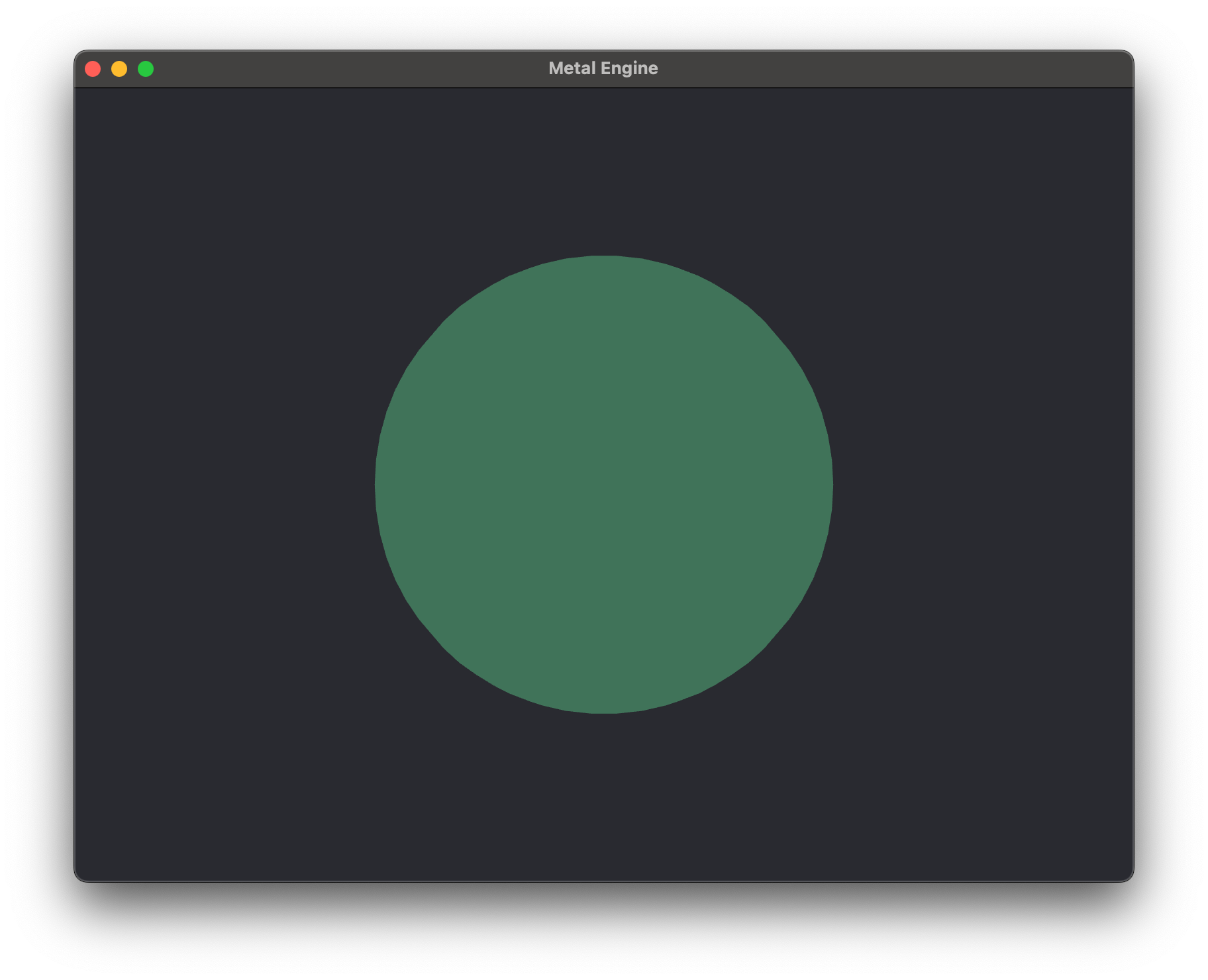
| Ambient |
|---|
 |
| Ambient + Diffuse |
 |
| Ambient + Diffuse + Specular |
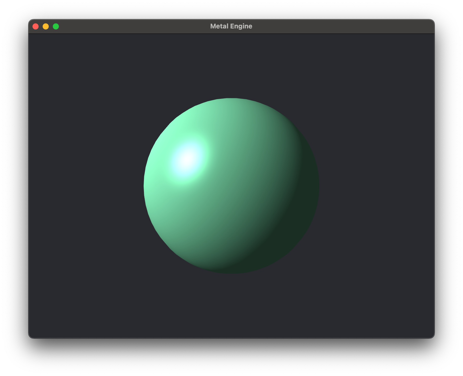 |
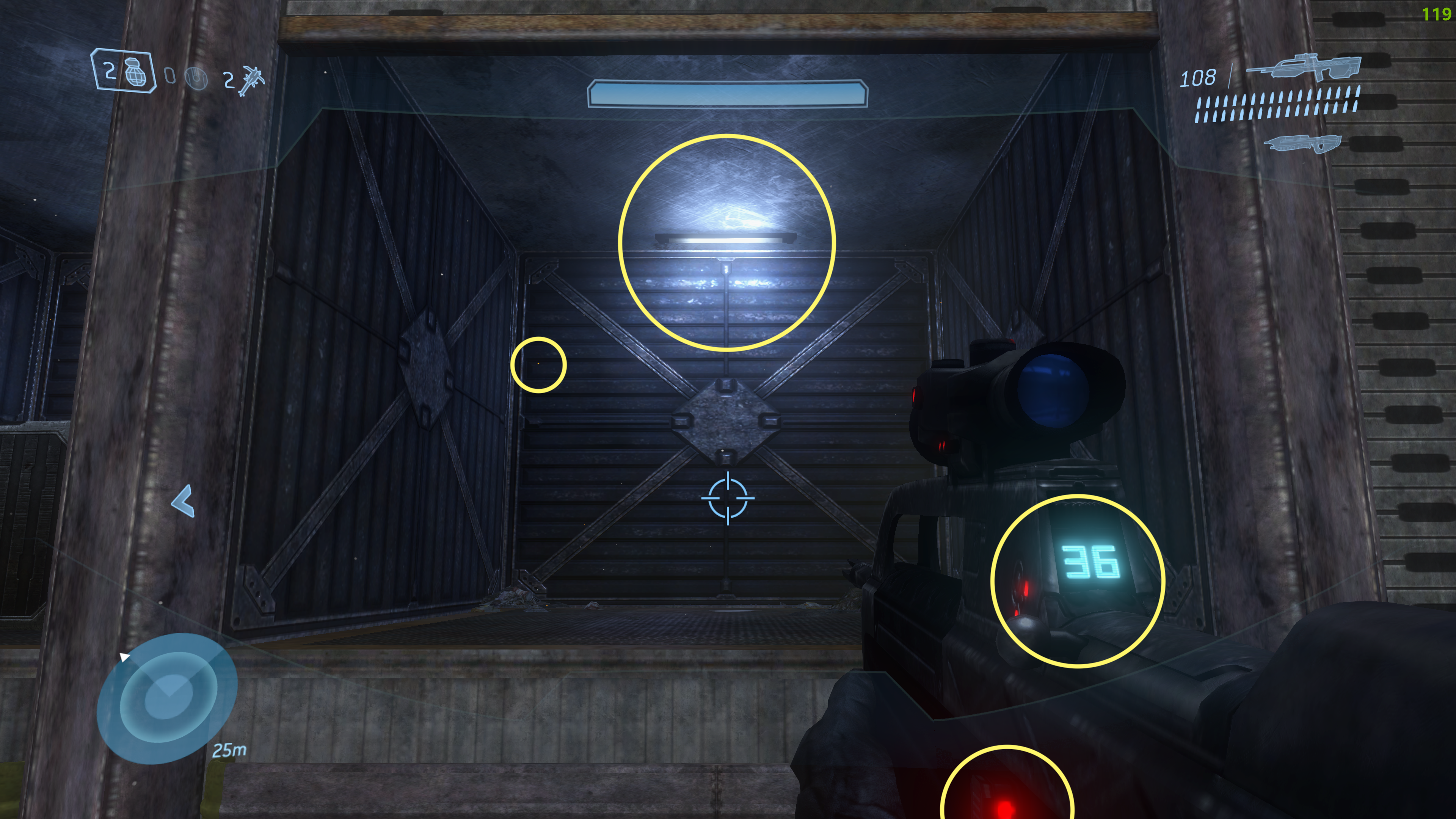
Above you can see 3 different examples, combining 3 of the basic lighting components, ambient, diffuse, and specular. Below you can see various examples of emissive lighting used in Halo 3. Notice that the light source at the top of the frame is affecting the lighting of the surrounding area as well. Typically this is an expensive effect that is usually approximated or pre-computed in real-time engines.
Emissive Example
Now, let's briefly discuss some of the major shading models that exist within Computer Graphics, as well as the differences between them, roughly ordered in increasing complexity:
- Flat Shading
- Gouraud Shading
- Phong Shading
- Blinn-Phong Shading
- Deferred Shading
- Phsyically Based Rendering (PBR)
- Ray-Tracing
Basic Shading Models
In summary, a lighting model is the overarching concept that dictates how different types of light and material interactions are simulated. The components like ambient, diffuse, specular, and others are the individual effects that the lighting model uses to compute the final appearance of surfaces in the scene.
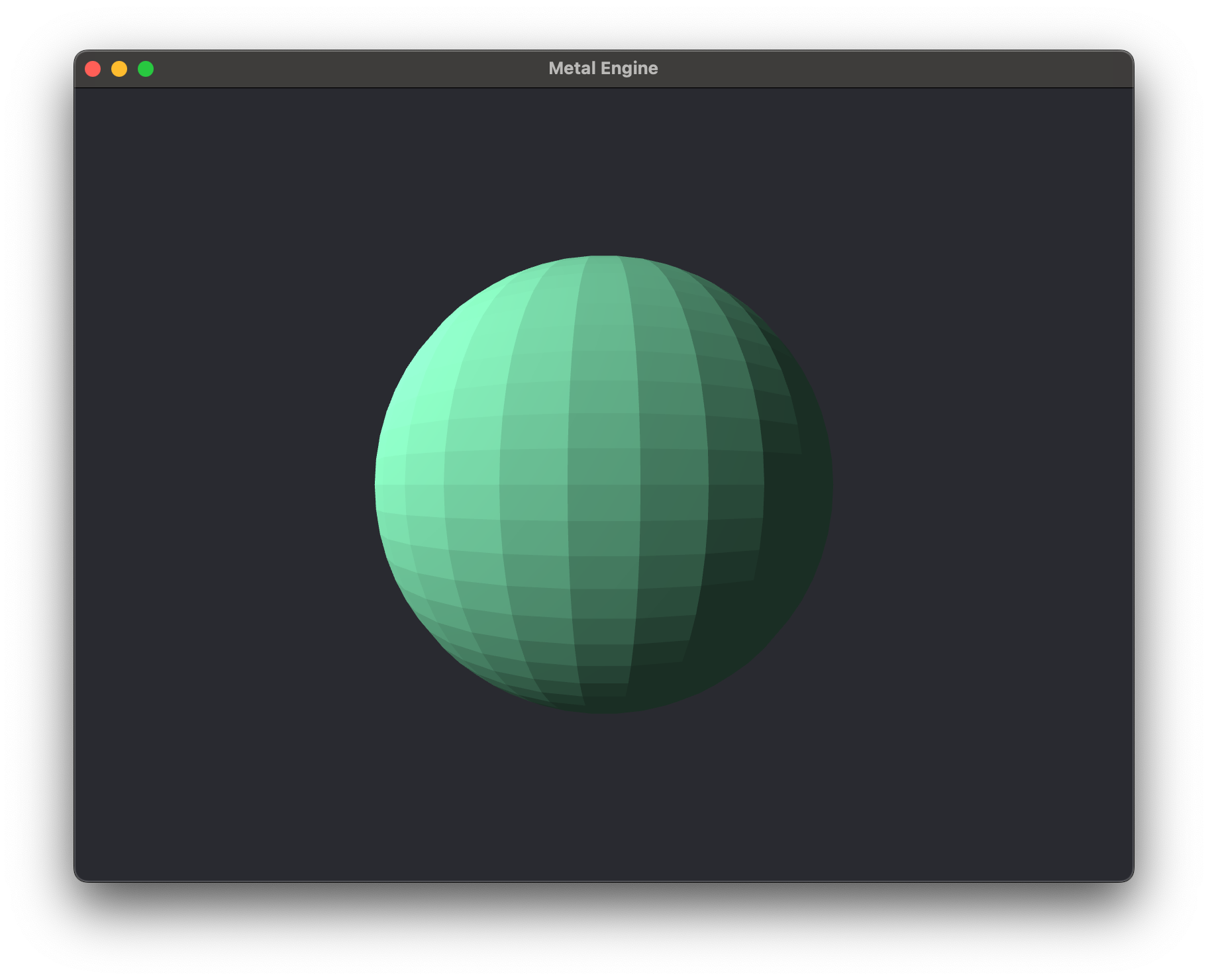
Flat Shading
Flat shading is the most basic form of shading used within Computer Graphics, and is often used when performance is a priority over visual quality or for a stylistic choice to give a low-poly retro look. It is typically done by calculating the lighting by using just one normal vector per face, the normal that is perpendicular to the face. As you can see from the image below, each polygon of the 3D model is shaded with just a single color, leading to this sort of faceted look. Flat shading combines the ambient and diffuse components to produce the final color of each face.
fragment float4 sphereFragmentShader(FragmentData fragment,
                                     constant float4& sphereColor,
                                     constant float4& lightColor,
                                     constant float4& lightPosition)
{

    // Ambient
    float ambientStrength = 0.2f;
    float4 ambient = ambientStrength * lightColor;

    // Diffuse
    float3 norm = normalize(fragment.normal.xyz);
    float4 lightDir = normalize(lightPosition - fragment.position);
    float diff = max(dot(norm, lightDir), 0.0);
    float4 diffuse = diff * lightColor;

    float4 finalColor = (ambient + diffuse) * sphereColor;

    return finalColor;
}
Gouraud Shading
Gouraud shading combines the ambient, diffuse, and specular lighting components, calculated at each vertex, and then interpolates these colors over the faces of the polygons. While this creates smoother transitions between light and dark areas, it can result in innacurate shading within the polygon, in particular for specular highlights.
vertex OutData sphereVertexShader(uint vertexID [[vertex_id]],
             constant VertexData* vertexData                 [[buffer(0)]],
             constant TransformationData* transformationData [[buffer(1)]],
             constant float4& sphereColor                      [[buffer(2)]],
             constant float4& lightColor                     [[buffer(3)]],
             constant float4& lightPosition                  [[buffer(4)]],
             constant float4& cameraPosition                 [[buffer(5)]])
{
    OutData out;
    out.position = transformationData->perspectiveMatrix * transformationData->viewMatrix * transformationData->modelMatrix * vertexData[vertexID].position;
    out.normal = vertexData[vertexID].normal;
    out.fragmentPosition = transformationData->modelMatrix * vertexData[vertexID].position;


    // Ambient
    float ambientStrength = 0.2f;
    float4 ambient = ambientStrength * lightColor;

    // Diffuse
    float3 norm = normalize(out.normal.xyz);
    float4 lightDir = normalize(lightPosition - out.fragmentPosition);
    float diff = max(dot(norm, lightDir.xyz), 0.0);
    float4 diffuse = diff * lightColor;

    // Specular
    float specularStrength = 1.0f;
    float4 viewDir = normalize(cameraPosition - out.fragmentPosition);
    float4 reflectDir = reflect(-lightDir, float4(norm, 1));
    float spec = pow(max(dot(viewDir, reflectDir), 0.0), 16);
    float4 specular = specularStrength * spec * lightColor;

    out.finalColor = (ambient + diffuse + specular) * sphereColor;

    return out;
}

fragment float4 sphereFragmentShader(OutData in [[stage_in]])
{

    return in.finalColor;
}

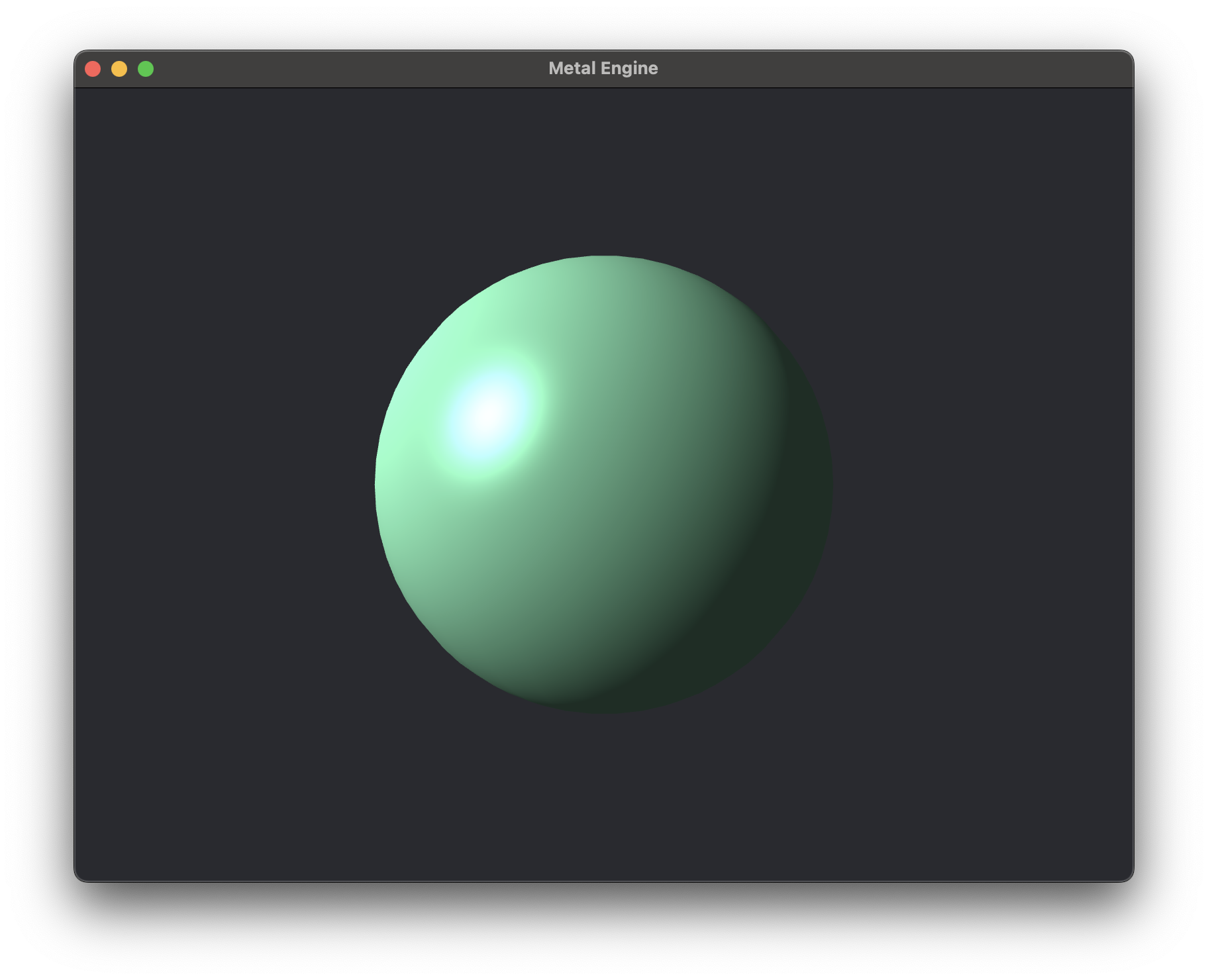
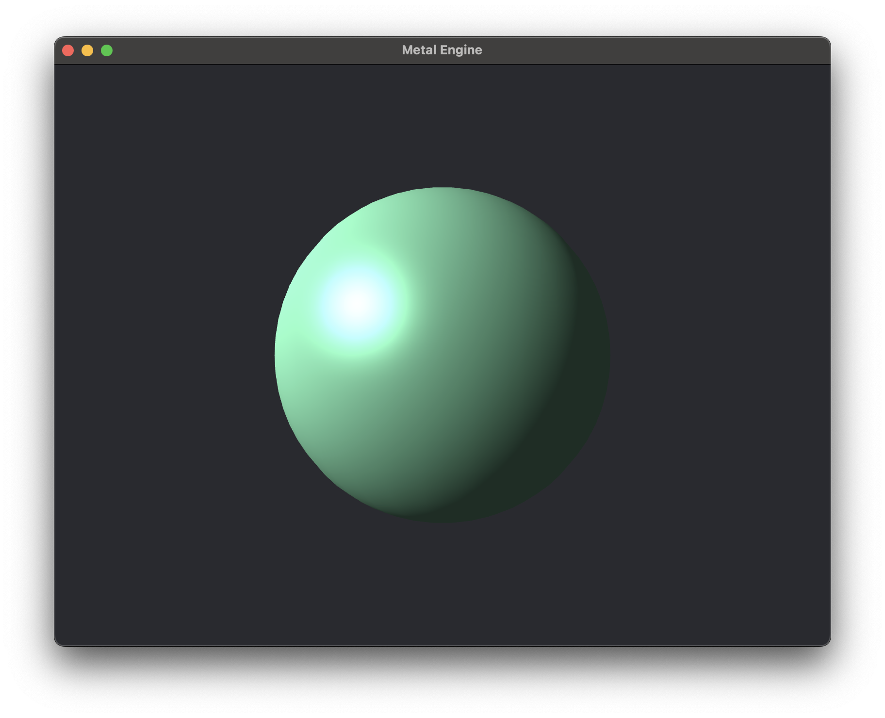
Phong Shading
Phong shading is very similar to Gouraud shading, combinging the same ambient, diffuse, and specular lighting components, but instead of interpolating the color between vertices, the normals are interpolated between the vertices and the light is evaluated per-pixel. This essentially produces an effect where the diffuse component and the specular highlights are calculated much more accurately that in the Gouraud shading model. The visual differences should be quite significant when comparing them.
fragment float4 sphereFragmentShader(OutData in [[stage_in]],
                                     constant float4& sphereColor                      [[buffer(0)]],
                                     constant float4& lightColor                     [[buffer(1)]],
                                     constant float4& lightPosition                  [[buffer(2)]],
                                     constant float4& cameraPosition                 [[buffer(3)]])
{

    // Ambient
    float ambientStrength = 0.2f;
    float4 ambient = ambientStrength * lightColor;

    // Diffuse
    float3 norm = normalize(in.normal.xyz);
    float4 lightDir = normalize(lightPosition - in.fragmentPosition);
    float diff = max(dot(norm, lightDir.xyz), 0.0);
    float4 diffuse = diff * lightColor;

    // Specular
    float specularStrength = 1.0f;
    float4 viewDir = normalize(cameraPosition - in.fragmentPosition);
    float4 reflectDir = reflect(-lightDir, float4(norm, 1));
    float spec = pow(max(dot(viewDir, reflectDir), 0.0), 16);
    float4 specular = specularStrength * spec * lightColor;

    float4 finalColor = (ambient + diffuse + specular) * sphereColor;
    return finalColor;
}
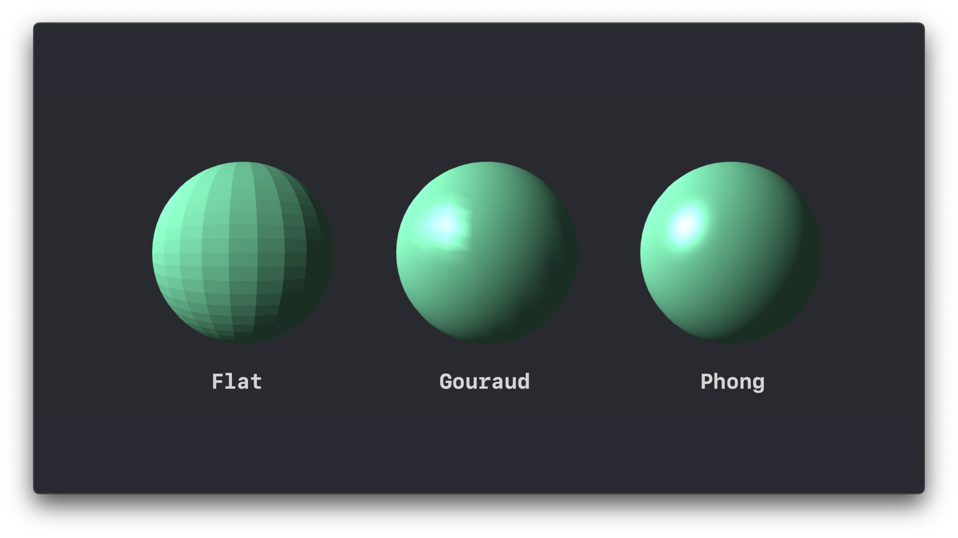
Flat vs Gouraud vs Phong Shading
Blinn-Phong Shading
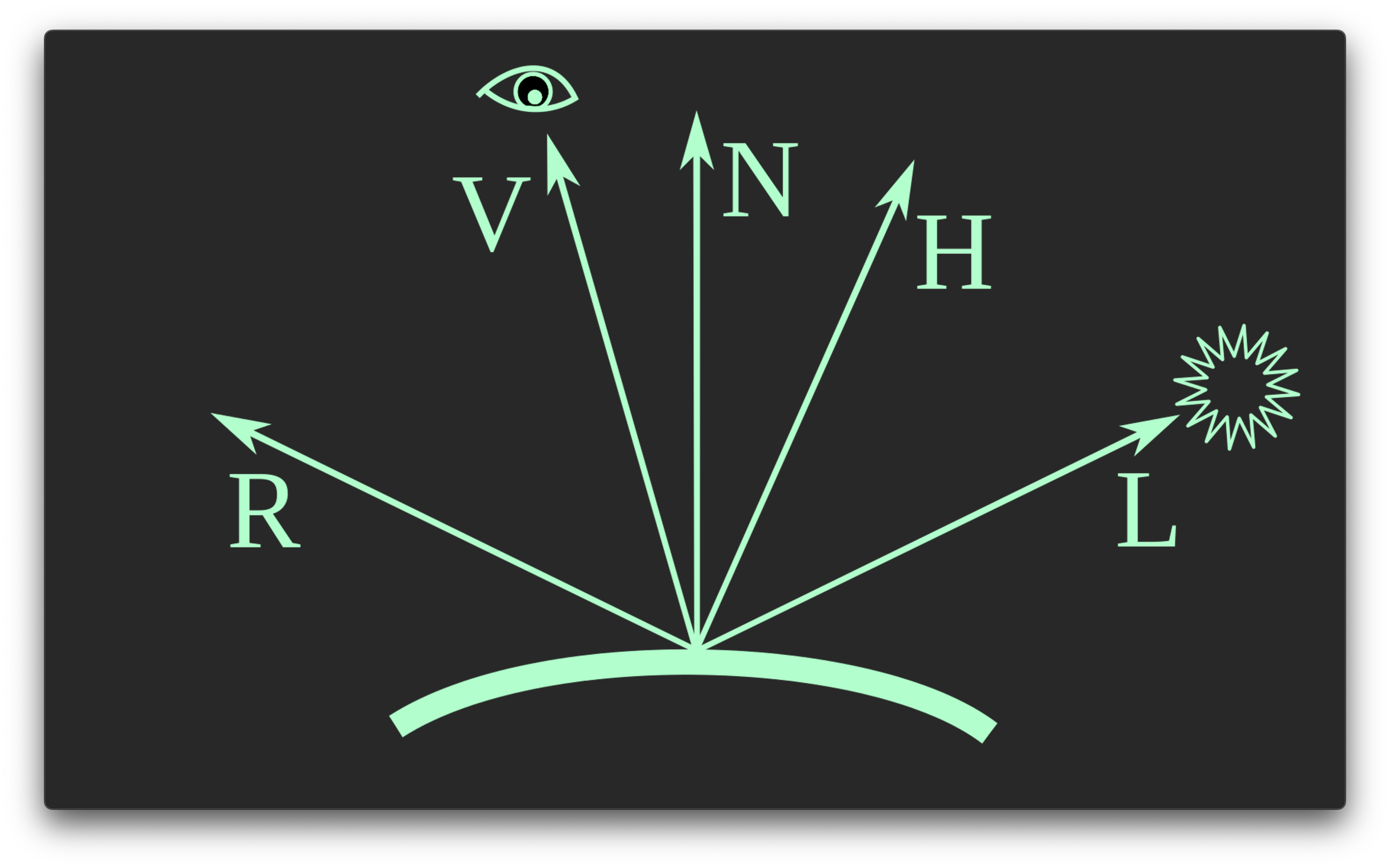
Phong Shading and Blinn-Phong Shading are both techniques that are used to simulate the way light interects with surfaces, specifically how light reflects to create specular highlights. Blinn-Phong is a modification to the Phong model that simplifies the specular calculation by using what is know as the halfway vector, i.e. the vector that lies halfway between the view and the light-source vectors.
Let's first break down the vectors for calculating the Phong and Blinn-Phong shading models.
-
\(L\) is the normalized vector pointing in the direction of the light source.
-
\(N\) is the vector normal to the surface at the fragment we are operating on.
-
\(V\) is the normalized view direction vector, pointing in the direction of the "view" or camera position.
-
\(R\) is the normalized reflection vector, which represents the direction a perfectly reflected light ray would take from our light source after hitting the surface of our object.
-
\(H\) is the normalized halfway vector, and it is the vector that lies halfway between the light direction vector, \(L\), and the view direction vector \(V\).
Let's compare the code snippets for calculating the specular component of the Phong and Blinn-Phong Models:
float3 reflection = normalize(reflect(-lightDirection, normal));
float specularIntensity = pow(max(dot(reflection, viewDirection), 0.0), shininess);
float3 specular = specularIntensity * lightColor;
- \(R = N \cdot 2*(L \cdot N) - L\)
- \(S_{Phong} = max(R \cdot V, 0)^a\)
We clamp the dot product between \(R\) and \(V\) to 0 to avoid negative values, which would not make physical sense.
float3 halfway = normalize(lightDirection + viewDirection);
float specularIntensity = pow(max(dot(normal, halfway), 0.0), shininess);
float3 specular = specularIntensity * lightColor;
- \(H\) = \(\dfrac{V+L}{||V+L||}\)
- \(S_{Phong} = max(N \cdot H, 0)^a\)
The big difference to note here, is that in Phong shading the calculation of the reflection vector is not free, and requires two dot products:
- \(R = N \cdot 2*(L \cdot N) - L\)
Calculation of the halfway vector in the Blinn-Phong model is more computationally efficient, as it's only an addition between two vectors, and overall it represents light more realistically than Phong for many types of surfaces.
Everything up until now will be covered in the code section of this chapter. For the following shading models which are much more complicated, I will simply give an overview of them and we will get to a more indepth discussion of them in the Advanced Chapters.
Advanced Shading Models
Deferred Shading
Deferred shading is a technique used in computer graphics to efficiently render complex scenes with multiple (or many) light sources by decoupling the lighting calculations from the geometry rendering process. The rendering we've done up until now is what's called foward rendering. In forward rendering, a fragment that isn't influenced by a light source still undergoes calculations for that light, wasting computational resources. Deferred rendering fixes this problem, and ensures that lighting calculations are only performed for fragments that are actually affected by each light source. A deferred shading pipeline splits rendering into two stages:
-
In the Geometry Pass, the scene's geometry gets rendered to a series of textures called the "G-Buffer" or "Geometry Buffer", where each texture is responsible for storing different types of data, such as the world-space coordinates, normal, diffuse, specular, depth, texture coordinates, etc.
-
Then, in the Lighting Pass, the scene is rendered again, but now each light is applied individually to the scene. For each light source, the shader will read the relevant data from the G-buffer and calculate the light's effect. Importantly, these calculations are only performed for pixels within the light's influence. How do figure that out? Well, this is typically done by rendering some sort of geometric volume that encompasses the light's effect range, like a sphere for a point light, or a cone for a spot-light, and then applying lighting calculations only within that volume.
The main benefit of deferred shading is that it significantly reduces the number of redundant lighting calculations. However, just like everything there are some downsides to consider:
- The Geometry Buffer requires storing a significant amount of data for each pixel, which can lead to high memory usage that only get sworse as resolution increases, and can become a limiting factor due to memory bandwith limitations, particularly on lower end hardware.
- Deferred rendering doesn't support Multi-Sample Anti-Aliasing (MSAA), one of the more common and efficient techniques to reduce aliasing, and in particular the one we discussed and implemented in the previous chapter. MSAA requires multiple samples per pixel to be stored before shading, which conflicts with this two-pass approach to rendering. If we wanted to use MSAA in a deferred renderer, we would have to store multiple samples per pixel for each texture in the G-buffer, which would greatly increase the memory usage and basically negate the performance benefits of deferred shading. To address aliasing, you have to rely on post-processing anti-aliasing techniques like Fast Approximate Anti-Aliasing (FXAA) or Temporal Anti-aliasing (TAA) which usually aren't as effective as standard MSAA.
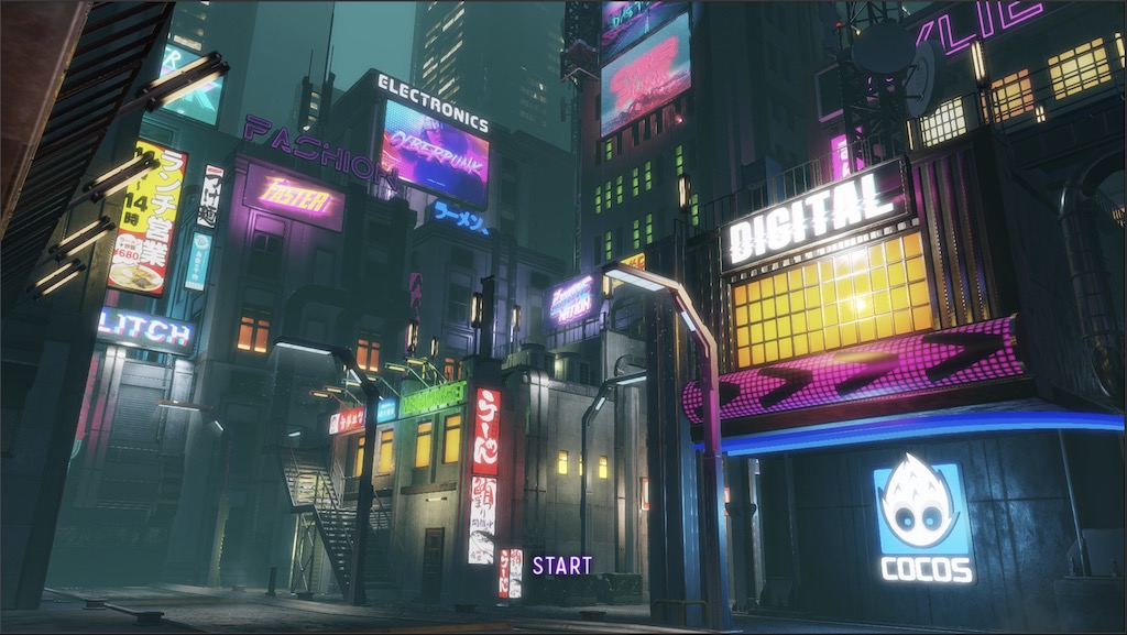
Below, I've included an example of a game scene that has many lights in it, which should give you an idea of what kind of environment it might be useful for.
If your interested in the specifics of how to create a deferred rendering pipeline, I'll be covering this soon in the Advanced Chapters. Stay tuned!
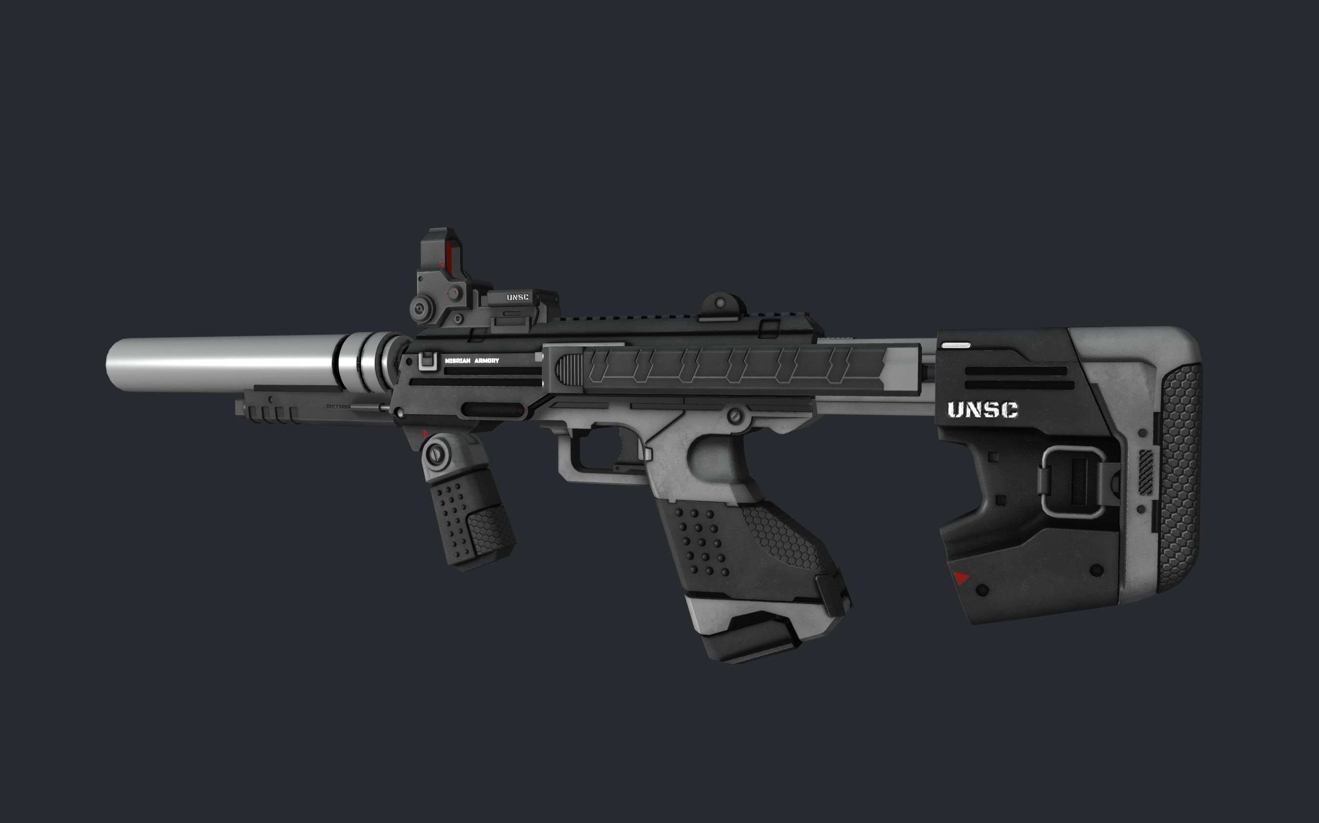
Physically Based Rendering (PBR)
Physically Based Rendering (PBR) is a rendering technique that aims to render things as realistically as possible by simulating the phsyical interaction between light and materials. It relies on theories of light reflection and material properties rooted in phsyics to ensure that materials behave consisetently under various conditions. PBR is a complex topic, and will require at least an entire chapters worth (or more) of explanation to get right, so I won't cover it in detail here. To give you a taste of what it's capable of, take a look at the same object rendered in our engine using Blinn-Phong Shading, versus the same object rendered in a PBR-based engine.
| Non-PBR |
|---|
 |
| PBR |
 |
Raytracing
Raytracing is a rendering technique that simulates the physical behaviour of light to create realistic images in our 3D graphics environments. The core principle involves casting rays of light from the camera into the scene to determine what is visible on the screen. For each pixel on the screen, we'll cast at least one ray. The more rays cast or "samples" we use per pixel, the more realistic our image will be.
When we cast a ray into the scene, we need to determine whether it will intersect with the geometry in our scene. This is called an intersection test, which is one of the fundamental operations done in ray-tracing. Although it sounds relatively simple, we have all sorts of techniques for speeding up this calculation, like Bounding Volume Hierarchies, which spatially sorts our geometry so rays can quickly discard large volumes of space of irrelevant geometry to perform an intersection test with. When a ray hits a surface, it can bounce around in different directions, dependent on the surface it encounters. Again, to achieve a more realistic result, we would usually want to have each ray bounce around multiple times. You can start to undestand why ray-tracing can get very computationally expensive. Imagine for each pixel on a 4k monitor, 3840 x 2160 = 8,294,400 pixels. If we bounce each ray off of our surfaces one time, that's over 160 million intersection tests per frame. When playing a game, we usually want to render more than 30 frames every second, so until recently ray-tracing in real time hasn't been feasible due to the limitations of our graphics hardware. This is starting to change of course, but we still have to use all sorts of fancy denoising algorithms to clean up our image. We also have image Super Sampling technique's like NVIDIA's Deep Learning Super Sampling (DLSS) allows us to render our game at a lower internal resolution and uses machine learning to upscale the final image to our monitor resolution as a way to improve rendering performance. And even then, most real-time raytracing applications are going to use a hybrid approach that combines traditional rasterization techniques like the one's we've discussed up until now with raytracing, where raytracing might only be used to render key visual elements like reflections, shadows, and global illumination.
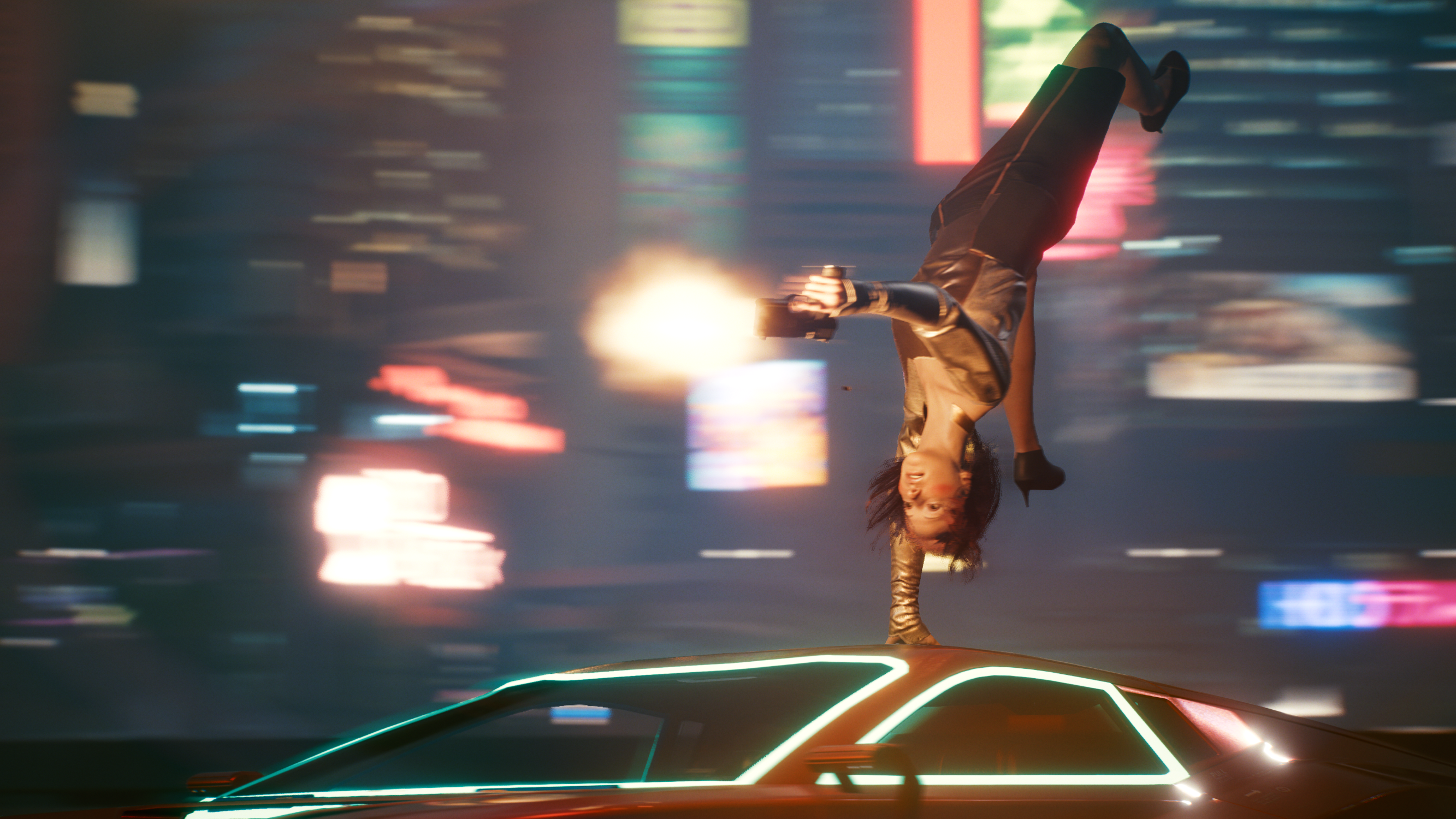
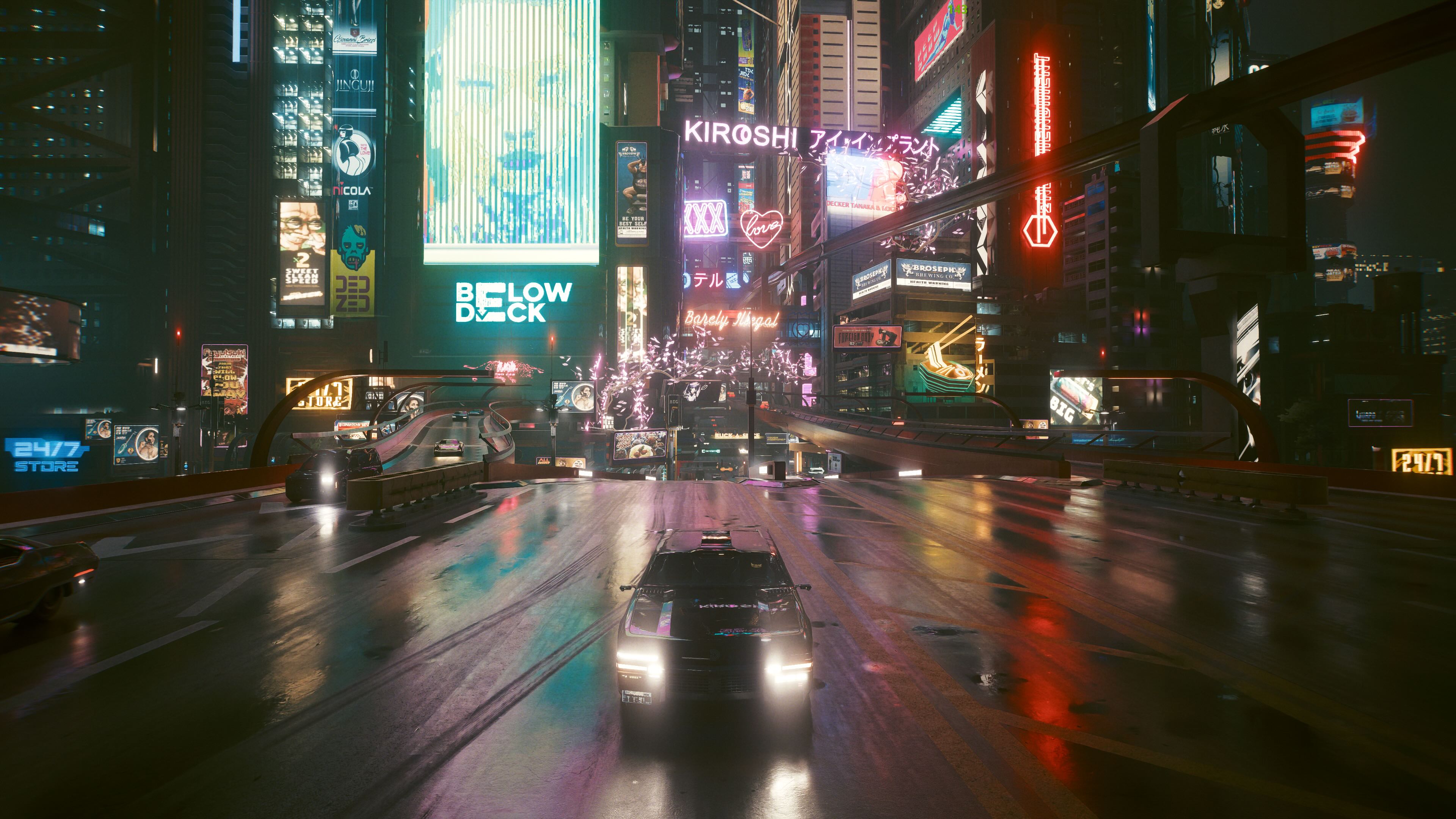
Below are some example screenshots I took from the gold standard for real-time raytracing in a videogame, Cyberpunk 2077. Pretty incredible, isn't it?
Raytracing
| Cyberpunk 2077 (rendered in real time) |
|---|
 |
 |
The Code - Phong and Blinn-Phong Shading
We're going to skip implementing Flat and Gouraud shading, because they're pretty lame. We'll start by implementing the Phong Shading model, and then we'll do the quick modification using the halfway vector to get Blinn-Phong shading.
...
Full write-up soon to come! For now, the code is accessible on the GitHub repository under branch Lesson_2_2, and here is the finished product: