Going 3D with Metal
Things will get a lot more interesting in this Chapter, as we're finally going 3D!
To do this, we'll need to add 3 important things to our rendering engine:
- A 3D Object to Render. For this chapter, we'll render a cube.
- Perspective Projection to add a sense of depth to our scene.
- A Depth Buffer for discarding non-visible fragments.
How will we create a cube? What is perspective projection? What is a... Depth Buffer? We'll discuss these topics in the following sections, as well as a few extra topics that will be useful for us as our scenes and objects get more complicated. Before diving in, if you are at all rusty with linear algebra concepts, and in particular matrices and basis vectors, I would highly recommend watching 3blue1brown's Linear Algebra series.
Creating a Cube
A cube happens to be a perfect progression from the square that we rendered in the previous chapter. It's a simple object, so we can define the vertices manually.
First, let's update the MTLEngine header file:
class MTLEngine {
    ...
private:
    ...
    MTL::Buffer* cubeVertexBuffer;
    MTL::Buffer* transformationBuffer;
}
VertexData.hpp file and add a struct calledTransformationData that will hold our model, view, and perspective matrices. If you're not sure what those are, I'll get into it later in the chapter:
#pragma once
#include <simd/simd.h>

using namespace simd;

struct VertexData {
    float4 position;
    float2 textureCoordinate;
};

struct TransformationData {
    float4x4 modelMatrix;
    float4x4 viewMatrix;
    float4x4 perspectiveMatrix;
};
For now, we'll define all 36 of our cube vertices manually. Just like in the last chapter, each face has 6 vertices, because our square is defined with two triangles. Each triangle of course has 3 vertices each. So, 3 vertices per triangle, 2 per face, 6 faces in total. That's 36 vertices of fun :), Lucky for you, I've defined vertices and texture coordinates for you:
void MTLEngine::createCube() {
    // Cube for use in a right-handed coordinate system with triangle faces
    // specified with a Counter-Clockwise winding order.
VertexData cubeVertices[] = {
        // Front face
        {{-0.5, -0.5, 0.5, 1.0}, {0.0, 0.0}},
        {{0.5, -0.5, 0.5, 1.0}, {1.0, 0.0}},
        {{0.5, 0.5, 0.5, 1.0}, {1.0, 1.0}},
        {{0.5, 0.5, 0.5, 1.0}, {1.0, 1.0}},
        {{-0.5, 0.5, 0.5, 1.0}, {0.0, 1.0}},
        {{-0.5, -0.5, 0.5, 1.0}, {0.0, 0.0}},

        // Back face
        {{0.5, -0.5, -0.5, 1.0}, {0.0, 0.0}},
        {{-0.5, -0.5, -0.5, 1.0}, {1.0, 0.0}},
        {{-0.5, 0.5, -0.5, 1.0}, {1.0, 1.0}},
        {{-0.5, 0.5, -0.5, 1.0}, {1.0, 1.0}},
        {{0.5, 0.5, -0.5, 1.0}, {0.0, 1.0}},
        {{0.5, -0.5, -0.5, 1.0}, {0.0, 0.0}},

        // Top face
        {{-0.5, 0.5, 0.5, 1.0}, {0.0, 0.0}},
        {{0.5, 0.5, 0.5, 1.0}, {1.0, 0.0}},
        {{0.5, 0.5, -0.5, 1.0}, {1.0, 1.0}},
        {{0.5, 0.5, -0.5, 1.0}, {1.0, 1.0}},
        {{-0.5, 0.5, -0.5, 1.0}, {0.0, 1.0}},
        {{-0.5, 0.5, 0.5, 1.0}, {0.0, 0.0}},

        // Bottom face
        {{-0.5, -0.5, -0.5, 1.0}, {0.0, 0.0}},
        {{0.5, -0.5, -0.5, 1.0}, {1.0, 0.0}},
        {{0.5, -0.5, 0.5, 1.0}, {1.0, 1.0}},
        {{0.5, -0.5, 0.5, 1.0}, {1.0, 1.0}},
        {{-0.5, -0.5, 0.5, 1.0}, {0.0, 1.0}},
        {{-0.5, -0.5, -0.5, 1.0}, {0.0, 0.0}},

        // Left face
        {{-0.5, -0.5, -0.5, 1.0}, {0.0, 0.0}},
        {{-0.5, -0.5, 0.5, 1.0}, {1.0, 0.0}},
        {{-0.5, 0.5, 0.5, 1.0}, {1.0, 1.0}},
        {{-0.5, 0.5, 0.5, 1.0}, {1.0, 1.0}},
        {{-0.5, 0.5, -0.5, 1.0}, {0.0, 1.0}},
        {{-0.5, -0.5, -0.5, 1.0}, {0.0, 0.0}},

        // Right face
        {{0.5, -0.5, 0.5, 1.0}, {0.0, 0.0}},
        {{0.5, -0.5, -0.5, 1.0}, {1.0, 0.0}},
        {{0.5, 0.5, -0.5, 1.0}, {1.0, 1.0}},
        {{0.5, 0.5, -0.5, 1.0}, {1.0, 1.0}},
        {{0.5, 0.5, 0.5, 1.0}, {0.0, 1.0}},
        {{0.5, -0.5, 0.5, 1.0}, {0.0, 0.0}},
    };

    cubeVertexBuffer = metalDevice->newBuffer(&cubeVertices, sizeof(cubeVertices), MTL::ResourceStorageModeShared);

    transformationBuffer = metalDevice->newBuffer(sizeof(TransformationData), MTL::ResourceStorageModeShared);

    // Make sure to change working directory to Metal-Tutorial root
    // directory via Product -> Scheme -> Edit Scheme -> Run -> Options
    grassTexture = new Texture("assets/mc_grass.jpeg", metalDevice);
}
Clockwise and Counter-Clockwise Winding Orders
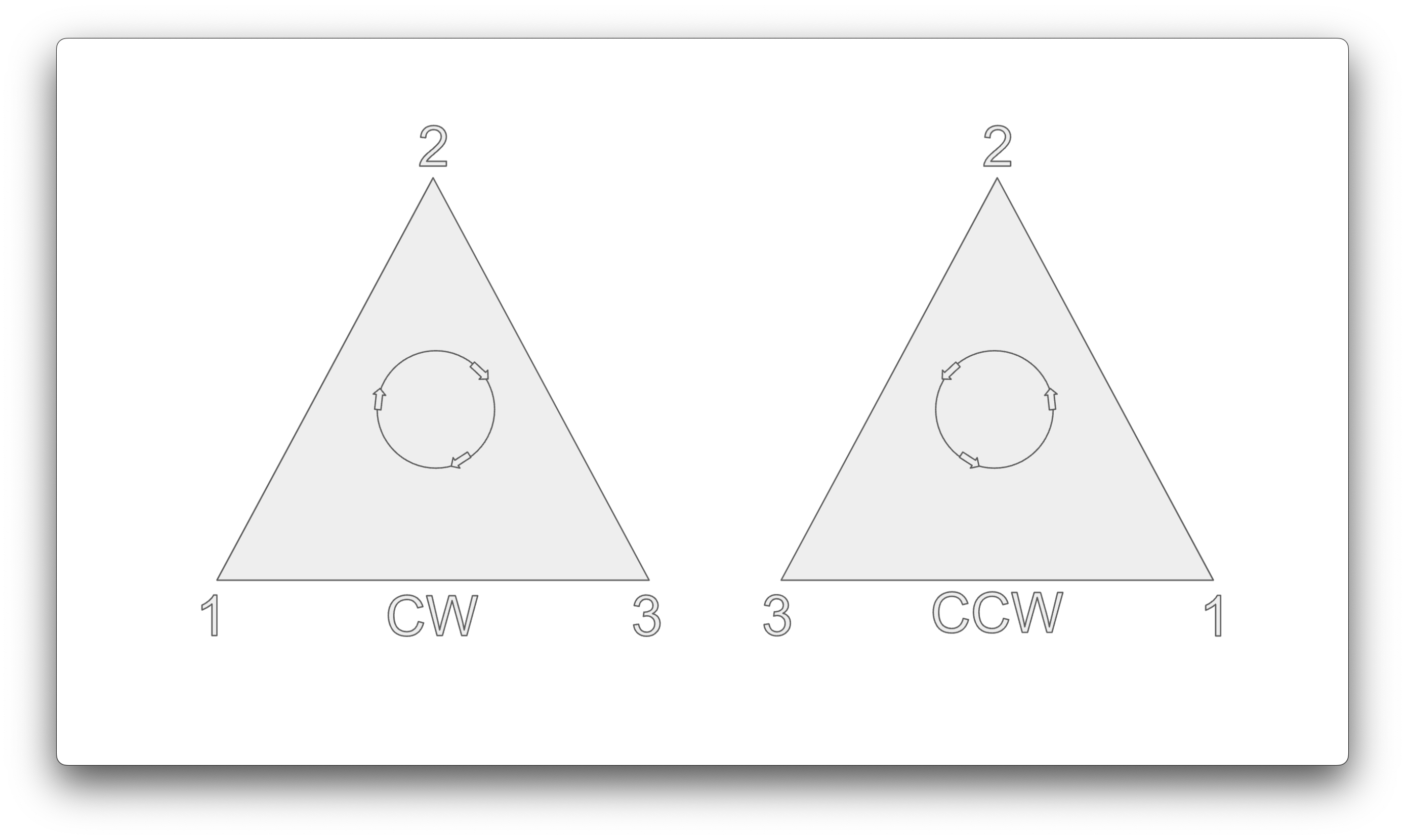
A triangle has 2 sides. In our case, we will instruct Metal to use the Counter Clockwise triangle winding order. The vertex winding order will determine which "face" or side of a given triangle corresponds to the front. Metal can then use this information to determine if a triangle face is facing towards or away from us, and cull (not render) it correspondingly. If a triangle is facing toward us we want to render it, as it will be unobstructed. If it's facing away from us, we can't see it, so we don't want to render it. Try to visualise the cube that we're going to be rendering. At any given time, we can only see at most 3 sides of it. That means that the remaining non-visible sides can be culled by Metal. Vertex winding order is important, as it gives us a cheap way to determine which triangles we don't need to render.
Another question to ask is, how do you know which winding order to choose? This depends on the coordinate system that you want to use for your rendering engine.
Choosing a Coordinate System
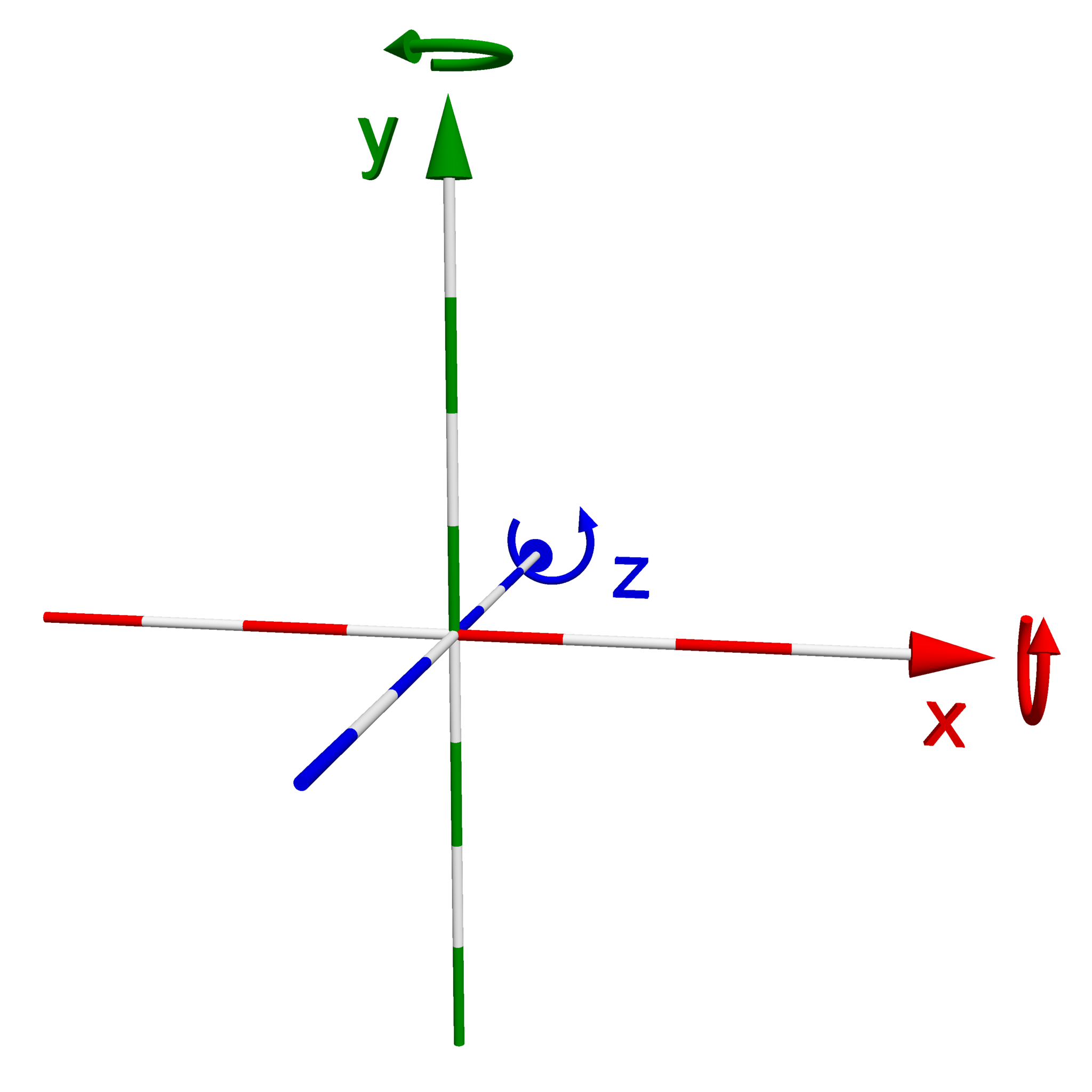
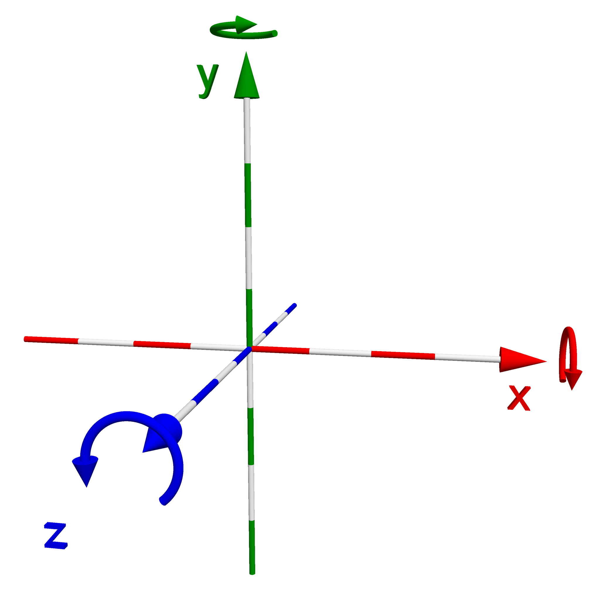
An important decision that we need to make when building a 3D rendering application is to choose a coordinate system to work with. What I mean by a “coordinate system” is, within the space where our objects and camera exists, what direction do we want our x, y, and z axis to point? The typical Cartesian coordinate system that you might be familiar with, we like to think of in the world of computer graphics as a “left-handed” coordinate system. In a left-handed coordinate system, the x-axis points to the right, the y-axis points up, and the z-axis points into your screen. If you hold your hand out in front of you and make an “L” shape with your thumb and index finger, these correspond to your x and y axis respectively. If you then point your middle finger out away from you, in the direction of your screen, this would correspond to the z-axis. If you do the same hand signal with your right hand, and then turn your hand around so that your middle finger points towards you, this should give you a visual representation of a “right-handed” coordinate system, where the positive z-axis (your middle finger) points towards us, out of the screen. Out of personal preference, I have decided to follow this coordinate convention throughout this tutorial series. Additionally, I’ve provided a visual below of the two coordinate systems I’ve described.
| Left-handed Coordinate System | Right-Handed Coordinate System |
|---|---|
 |
 |
There are some important ramifications that we should be aware of when choosing to work with a right or left-handed coordinate system.
- Direction of the result of the cross-product of two vectors. When using a right-handed coordinate system, we follow something called the right-hand rule. As an example, image that we have two vectors of length one (aka, unit vectors) that lie on the x-axis and y-axis pictured in the right-handed coordinate system above: \({V}_1 = (1, 0, 0)\), \({V}_2 = (0, 1, 0)\). To get another unit vector that points in the direction of the z-axis, we want to do \({V}_1 \times {V}_2\). Notice the order I've specified the cross product in here, try making a sweeping motion with your fingers from vector \({V}_1\) in the direction of vector \({V}_2\), it should match the counter-clockwise rotation displayed for the z-axis. This is the same thing that Metal will do behind the scenes to determine the front and back face triangles of your 3D models when we instruct it to use a Counter Clockwise winding order for our vertices.
- The winding order, or order in which you specify your vertices can impact how the object is rendered. In a right-handed coordinate system, we typically use a counter-clockwise winding order for our vertices, which allows us to easily determine whether a face is “front-facing”, facing towards us, or “back-facing” facing away from us, allowing Metal to easily discard and not render faces pointing away from us.
- The normal vector for a face is calculated using the cross product of two edge vectors from the polygon. Normals are essential for various rendering techniques such as lighting calculations.
- Looking Direction: In a right-handed system, the camera typically looks down the negative z-axis by default, whereas in a left-handed system the camera typically looks down the positive z-axis.
- Transformation matrices will slightly differ, like the perspective projection matrix. Or, if you choose to rotate an object around a particular axis, the direction of rotation will be flipped in a right versus left handed system, as you can see in the diagram above.
Transformations
Now that we have decided what kind of coordinate system we want to use, we need to discuss the series of transformations that our objects will go through to be rendered on the screen. Typically when you import a model into your rendering engine, the coordinates that are provided will center the object at the origin. Take our cube for example, we defined it to be centered at the origin. We call this initial coordinate space for each model, the aptly named “model-space”. If we imagine a scene in a game, it’s usually going to have all sorts of objects scattered throughout the scene, perhaps looking something like in the image below:
This mean's that we need some way to be able to move our objects around in space. Luckily, we can use affine transformations in the form of four dimensional matrices to do this. Using these, we can easily scale, translate, rotate, and sheer our vertices in space. I'll get a little bit more into the specifics in the Mathematics section of this chapter. When we scale, manipulate, or otherwise move our objects from their initial position/orientation in "model-space" to our desired position within the world, we say that these objects are now in "world-space". That’s great, we’ve now oriented everything properly in our scene, but, how do we view it from our camera’s perspective, like in the image above? Well, your camera, much like the objects in your scene will also have a position and an orientation within the world or “world-space”. In order to view everything from our camera’s perspective, we’re going to apply another matrix transformation called the “view” or sometimes the “camera” transformation. The key thing to realize here is that, we aren’t actually moving around any of the objects in the scene with the view transformation. We are simply applying a change of basis transformation to our world-space coordinates, along with a translation to move the origin of our world to the camera’s current position. This new “view-space” coordinate system is defined by three vectors that we define our camera to have, as well as the position of the camera in world-space:
- Forward Vector (F): Points in the direction the camera is looking.
- Right Vector (R): Points to the right of the camera.
- Up Vector (U): Points above the camera.
- Camera Position (P): The Position of the camera in World-Space.
A common form for the view matrix \( M_{view} \) used in a right-handed coordinate system is as follows:
The resulting view-space matrix will combine a change of basis matrix defined by our Forward, Right, and Up vectors, with a translation matrix that moves the origin of the world to the camera’s position. Now that our vertices are in view-space, the coordinate-space defined by our camera's position and orientation, we are ready to apply the perspective projection matrix. The perspective projection matrix is defined by the coordinate-system that we originally chose to work with, being a right-handed coordinate system, as well as the field of view (fov) of our camera, the aspect-ratio of our window, as well as a near and far clipping plane. In essence, each vertex on each model in our scene will go through this series of transformations to end up as a position in clip-space:
Once our vertex positions have been transformed to clip-space, our job is done, and Metal will clip or cull objects outside of the viewing frustum, and clip objects to the viewing frustum. It will then automatically perform the perspective or "homogenous" divide on each of our coordinates, transforming it to the final coordinate space called Normalized Device Coordinates. Well, what does all of that mean? We're going to get to that in the next section.
What is Perspective Projection?
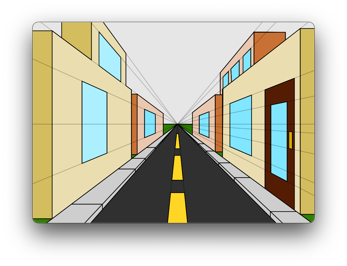
With our coordinate system chosen and our Cube now defined, we have to discuss the topic of Perspective Projection. In the context of 3D Computer Graphics, perspective projection is a technique used to represent a three-dimensional object on a two-dimensional plane, being our computer screen, mimicking the way our eyes perceive depth and scale. Essentially, we'll want to map 3D points in the world to 2D points on a rendering surface called the “viewing” or “projection” plane (which ends up being displayed on your computer screen), while maintaining the perception of “depth". Objects that are farther away from the camera appear smaller on the viewing plane, and parallel lines converge to a single point in the distance, known as the vanishing point.
Getting objects to appear on our screen and mimic the way they appear in real life is a pretty involved process. There are a lot of different steps to it, and if you aren’t familiar with the concept of “perspective projection” within the context of a 3D graphics pipeline, don’t worry about it too much. It may take a little while to wrap your head around the entire process, so you can always feel free to just follow along with the code and try to understand it as you go along.
Various Types of Projection Visualized
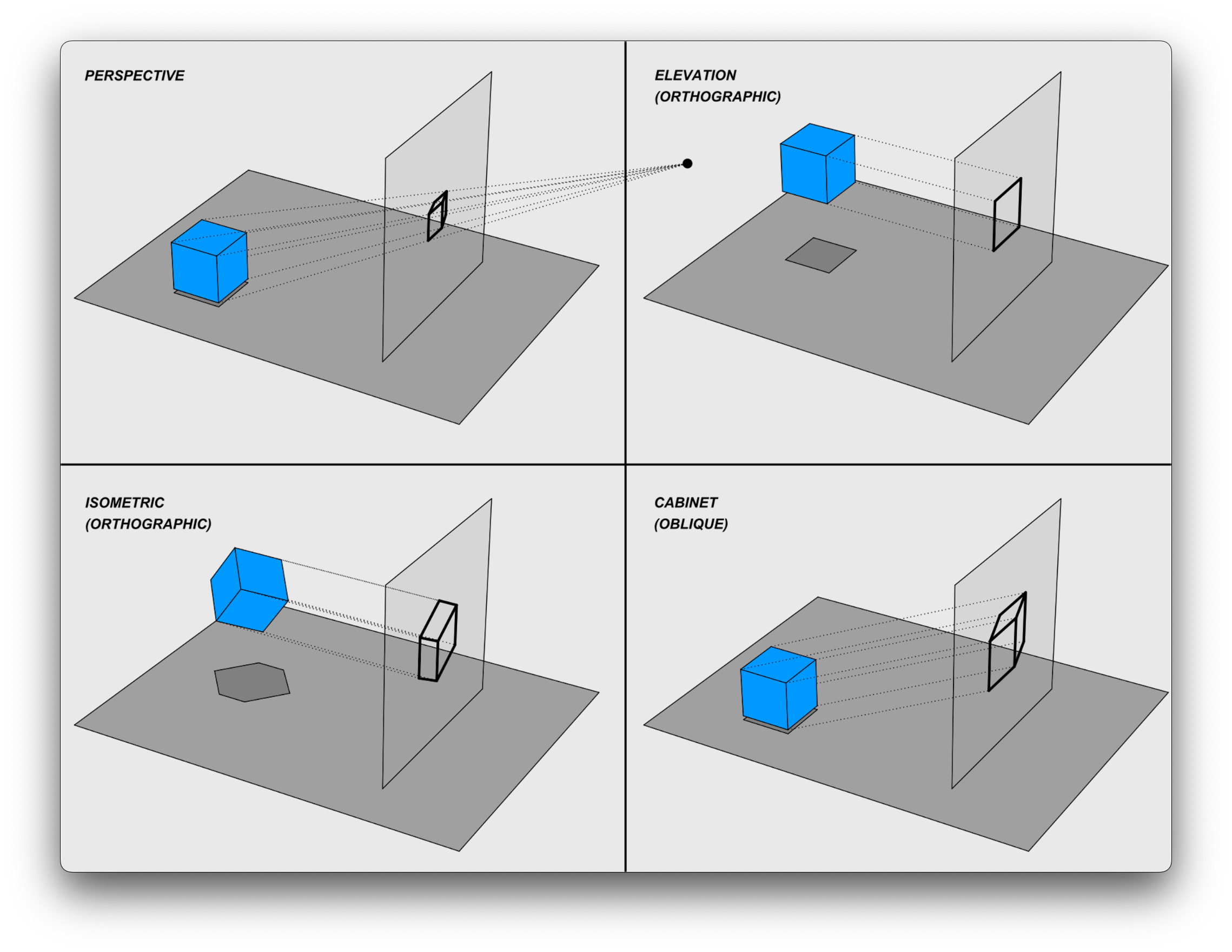 In reality, there are a variety of ways to map or "project" 3D points onto a 2D surface, and they have different purposes. In our case, we're trying to simulate how we would perceive things in real life using perspective projection. The further an object is away from us, the smaller we want it to appear on our screen, and vice versa as it gets closer to us. If we were an architect however, we might choose instead to use an orthographic projection to visualize our architectural drawings. Orthographic projections map our 3D points straight onto the viewing plane without any regard for the distance away, and so they are widely used in various fields such as engineering, architecture, design, and art for their ability to represent 3D objects accurately and without distortion. They are especially useful in situations where it's essential to maintain the exact dimensions and shapes of the objects being depicted.
Isometric Projection Visualised
Perspective Projection Visualised
Mathematics Behind Perspective Projection
Perspective projection can be represented mathematically by a 4D transformation matrix. We’ll use this perspective projection matrix to transform a point from what are called “homogenous” coordinates to it’s 2D screen position. In the context of 3D graphics, a vertex position in 3D space that would typically be represented with Cartesian coordinates (x, y, z) can be represented in 4D “homogenous” coordinates as (x, y, z, w).
Why are they useful?
- Unified Representation: Homogeneous coordinates allow for a unified representation of translation, rotation, scaling, and other affine transformations as matrix multiplications. Without our 4D homogeneous coordinates, translation of our 3D objects would not be possible through matrix multiplication alone.
- Perspective Projection: They are crucial for perspective transformations. The division by w (known as the homogeneous divide or the perspective divide) allows for points to be moved closer or farther away from the camera, effectively simulating perspective.
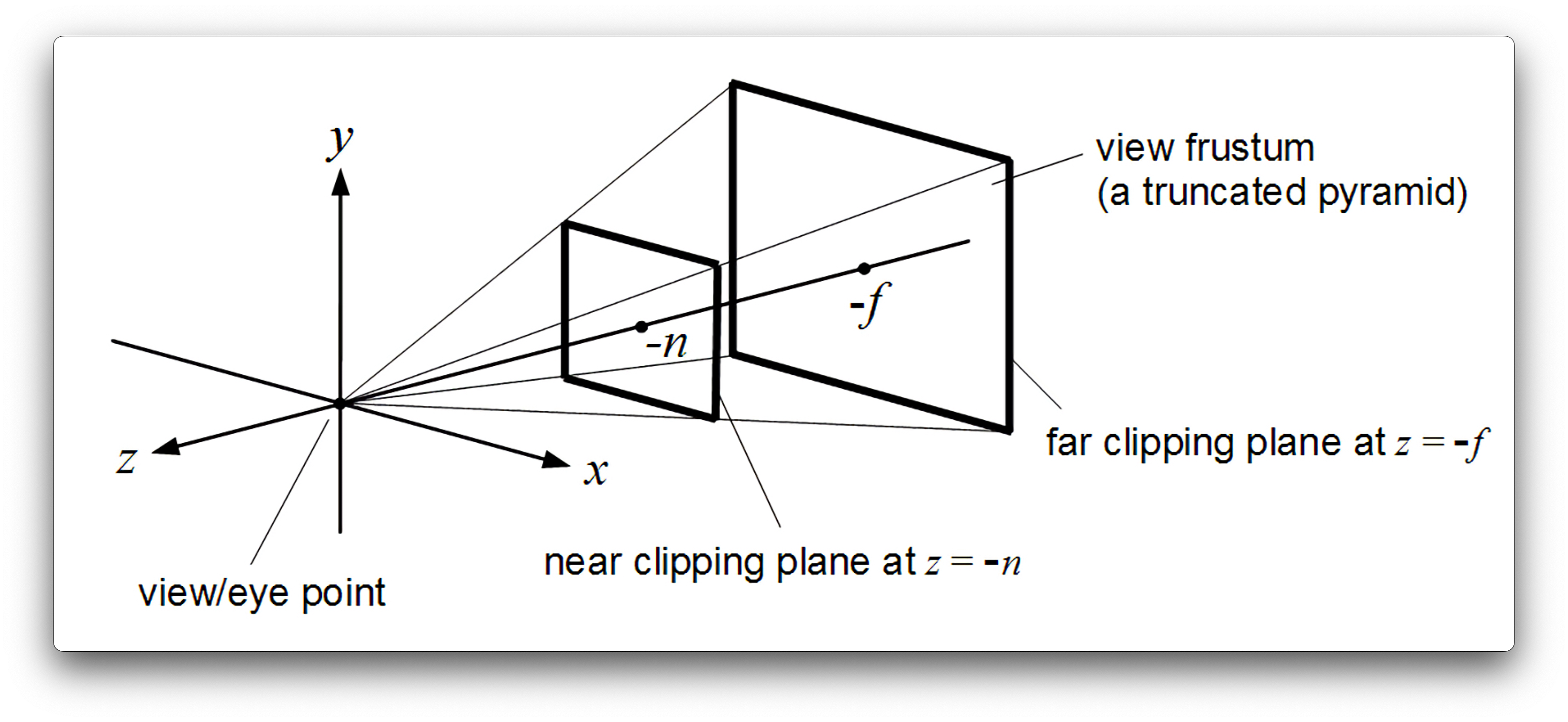
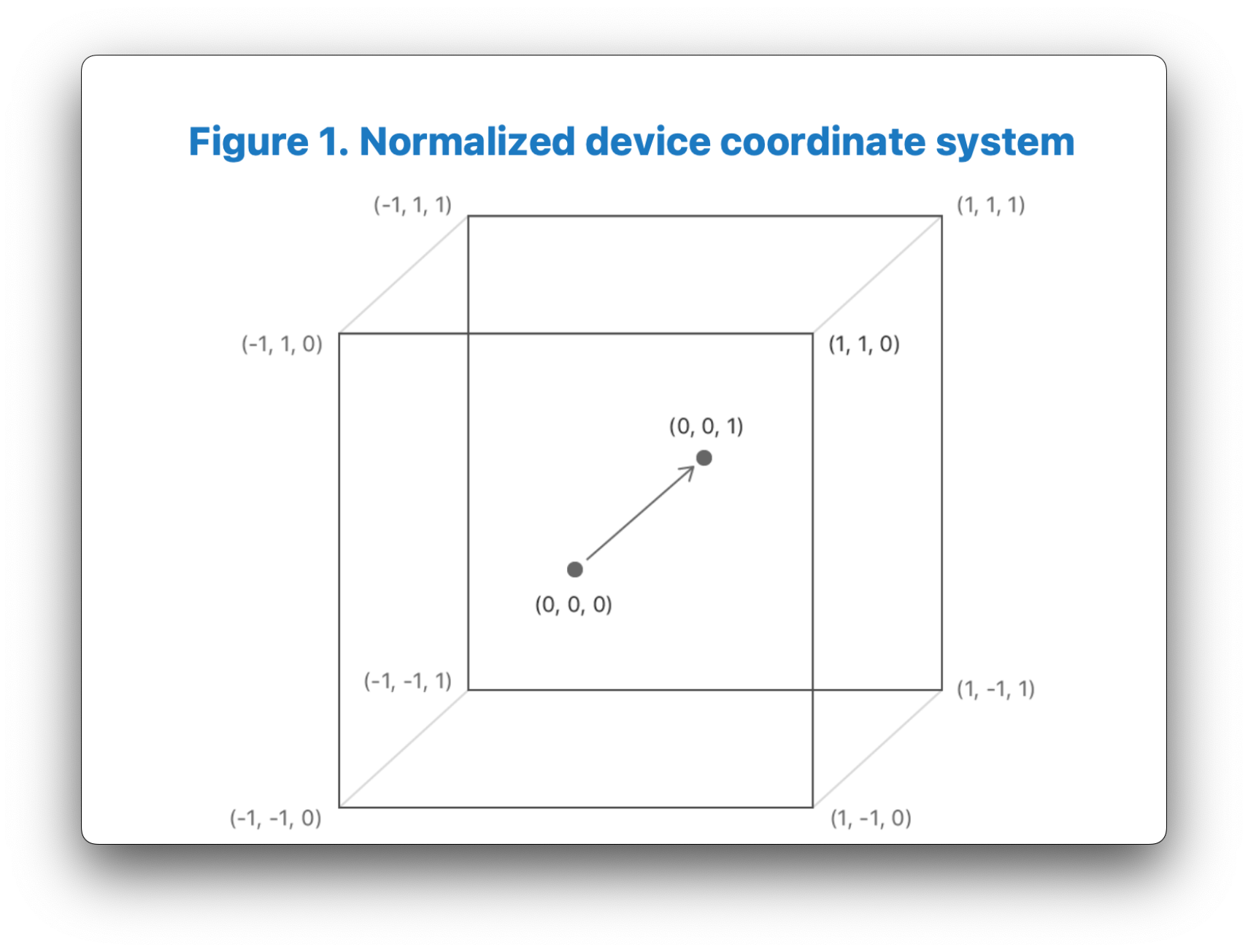
The perspective projection matrix takes in a variety of parameters, such as the field of view of your camera, the aspect ratio of the window/screen that you are rendering too, as well as the nearZ and farZ clipping planes. Based on these parameters, the perspective projection matrix creates what is called a “viewing frustum”, essentially a rectangular pyramid around your scene that represents what you can see, originating from the camera’s location. When you apply this perspective projection transformation matrix to your vertices, it essentially warps this pyramid-like viewing frustum into a cube shape that we call “clip-space”. When you apply the perspective projection matrix, the range of your x, y and z coordinates will be between [-w, w]. The w-component of your homogenous coordinate is manipulated in such a way that Metal will then divide our x, y, and z coordinates by the w-component automatically to normalize the range of our x, y, and z coordinates to Normalized Device Coordinate (NDC) space. In Metal, NDC is a left-handed coordinate system that ranges from [-1,1] in the x and y direction, and from [0,1] in the z direction. Having this normalized box-like shape allows us to easily test whether vertices in our scene are in or outside of the box, and discard or “cull” them appropriately, as we don’t want to render anything we can’t see. If you have half of an object inside the NDC box and half outside, then it will “clip” the object to the edge of the box, creating new vertices for the object along the box's edge.
In our engine, we'll use a right-hand perpsective projection matrix that will take in the field of view specified as an angle in radians (e.g. 90 * PI/2), the aspect ratio of our window (width/height), as well as the distance of the near and far clipping planes from the camera:
matrix_float4x4 matrix_perspective_right_hand(float fovyRadians,
                                              float aspect,
                                              float nearZ,
                                              float farZ)
{
    float ys = 1 / tanf(fovyRadians * 0.5);
    float xs = ys / aspect;
    float zs = farZ / (nearZ - farZ);
    return matrix_make_rows(xs,  0,  0,          0,
                             0, ys,  0,          0,
                             0,  0, zs, nearZ * zs,
                             0,  0, -1,          0 );
}
Putting It All Together
I think it’s best to explain the series of transformations that our vertices will go through in order to be projected onto the screen with an example. Let's imagine we have a square that we want to render. Imagine it is positioned initially at the origin, aligned with the \(xz\) plane. The 4 homogenous vertices defining the square are:
Step 1: Defining the Square in Model Space
- \( A_{model} = [ -1, 0, -1, 1 ] \)
- \( B_{model} = [ 1, 0, -1, 1 ] \)
- \( C_{model} = [ 1, 0, 1, 1 ] \)
- \( D_{model} = [ -1, 0, 1, 1 ] \)
Step 2: Model Transformation (Translation)
We'll move the square down the negative \(z\)-axis by two units. This requires a translation operation, represented by a translation matrix:
Multiplying each point by this matrix, we get these translated points in world-space:
- \( A_{world} = [ -1, 0, -3, 1] = M_{translation} \times A_{model} \)
- \( B_{world} = [ 1, 0, -3, 1] = M_{translation} \times B_{model} \)
- \( C_{world} = [ 1, 0, -1, 1] = M_{translation} \times C_{model} \)
- \( D_{world} = [ -1, 0, -1, 1] = M_{translation} \times D_{model} \)
Step 3: View Transformation
To construct a view matrix, you'll need three orthogonal unit vectors. A unit vector is a vector that has a magnitude of 1. In other words, it is a vector that points in a certain direction but has been normalized to have a length of 1.
- Forward Vector (F): Points in the direction the camera is looking.
- Right Vector (R): Points to the right of the camera.
- Up Vector (U): Points above the camera.
You'll also need the camera's position vector \( P \).
- Camera Position (P): The Position of the camera in World-Space.
A common form for the view matrix \( M_{view} \) used in a right-handed coordinate system is as follows:
We'll define our Forward, Right, and Up vectors, as well as the camera position like so:
- \(F = (1, 0, 0) \)
- \(R = (0, 1, 0) \)
- \(U = (0, 0,-1) \)
- \(P = (0, 1, 1) \)
This will give us the resulting view vector:
When we apply this view transformation matrix to our square vertices we get:
- \( A_{view} = [ -1, -1, -4, 1] = M_{view} \times A_{world} \)
- \( B_{view} = [ 1, -1, -4, 1] = M_{view} \times B_{world} \)
- \( C_{view} = [ 1, -1, -2, 1] = M_{view} \times C_{world} \)
- \( D_{view} = [ -1, -1, -2, 1] = M_{view} \times D_{world} \)
Remember, these are the coordinates of the square in the coordinate space oriented in the direction of the camera, where the camera's position is the new origin. The camera was positioned at \(P = (0, 1, 1)\) on the \(z\)-axis, so when we move the original origin to the camera's position, it's as though everything has been shifted in the opposite direction. Essentially, we move the square by one unit in the direction of the negative z-axis and negative y-axis.
Step 4: Perspective Transformation
Let's use a simplified perspective projection matrix for this example. We'll ignore aspect ratio and the far plane, focusing only on the near plane, which is at \(z = -1\). However, to make perspective account for Metal's NDC, we need to modify the z-coordinates in the perspective transformation. Given the original perspective matrix:
Our resulting perspective projection matrix becomes:
The third row third column's -0.5 scales the z-coordinate to half its value, and the -0.5 at the end of the third row translates the z-coordinate so it's in the range [0, 1] after the perspective divide.
Multiplying each point by this matrix, we get:
- \( A_{clip} = [ -1, -1, 1.5, 4 ] = M_{Metal} \times A_{view} \)
- \( B_{clip} = [ 1, -1, 1.5, 4 ] = M_{Metal} \times B_{view} \)
- \( C_{clip} = [ 1, -1, 0.5, 2 ] = M_{Metal} \times C_{view} \)
- \( D_{clip} = [ -1, -1, 0.5, 2 ] = M_{Metal} \times D_{view} \)
Step 5: Transform to NDC
To transform our vertices to NDC, Metal will automatically divide their respective x, y and z components by their w component, leaving us with:
- \( A_{NDC} = ( -0.25, -0.25, 0.375) \)
- \( B_{NDC} = ( 0.25, -0.25, 0.375) \)
- \( C_{NDC} = ( 0.5, -0.5, 0.25) \)
- \( D_{NDC} = ( -0.5, -0.5, 0.25) \)
After the perspective divide, the points are in normalized device coordinates. In this example, you can see that the \( x \) coordinates of points A and B are now closer to the origin (scaled down to \( \pm 0.25 \)) compared to points C and D (\( \pm 0.5 \)). This is because points A and B are positioned farther away in world-space from the camera (at \( z = -3 \), and so take on a larger w-component) compared to points C and D (at \( z = -1 \)). Notice how the division by the w component is what caused this "squishing" that perspective provides.
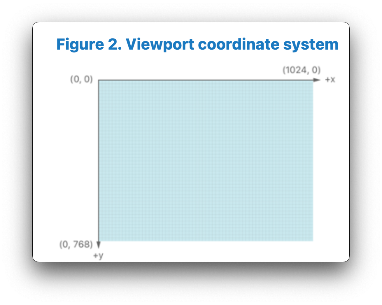
Step 6: The Viewport Transform
In Metal, the rasterizer stage is responsible for transforming our Normalized-device coordinates (NDC) into viewport coordinates, which correspond to pixels on our screen. The (x,y) coordinates in the viewport are measured in pixels, with the origin placed in the top-left corner of the viewport. Metal will take our NDC coordinates x and y values and scale them by the width and height of the screen respectively, to end up between (0, screen width) in the x-direction, and (0, screen height) in the y-direction:
Below is a visual representation of the viewport coordinate system used in Metal, borrowed from the Metal Shading Language Specification:
Step 7: Rasterization
After our square goes through this series of transformations to end up in NDC coordinates, the rasterizer stage transforms our vertices into screen space. The rasterizer then takes these vertices and determines which pixels on the screen they cover. This process is called rasterization. The result is a set of fragments. Each fragment corresponds to a potential pixel on the screen and carries with it interpolated data from the vertices, such as color, texture coordinates, and depth.
Result
When we put it all together, our scene might look a little something like this:
Hopefully this walkthrough has helped demonstrate the effects of each of the steps that our vertices go through, including perspective projection and the the significance of the homogenous coordinates mathematically.
Continuing with the Code
For convenience, we're going to add two new files provided by Apple to our project: AAPLMathUtilities.cpp and AAPLMathUtilities.h. We'll include the header in mtl_engine.hpp:
Since we've already defined our Cube and created our cubeVertexBuffer as well as our transformationBuffer, we can now define our model, view, and perspective projection matrices:
void MTLEngine::encodeRenderCommand(MTL::RenderCommandEncoder* renderCommandEncoder) {
    // Moves the Cube 2 units down the negative Z-axis
    matrix_float4x4 translationMatrix = matrix4x4_translation(0, 0,-1.0);

    float angleInDegrees = glfwGetTime()/2.0 * 45;
    float angleInRadians = angleInDegrees * M_PI / 180.0f;
    matrix_float4x4 rotationMatrix = matrix4x4_rotation(angleInRadians, 0.0, 1.0, 0.0);

    matrix_float4x4 modelMatrix = simd_mul(translationMatrix, rotationMatrix);

    simd::float3 R = simd::float3 {1, 0, 0}; // Unit-Right
    simd::float3 U = simd::float3 {0, 1, 0}; // Unit-Up
    simd::float3 F = simd::float3 {0, 0,-1}; // Unit-Forward
    simd::float3 P = simd::float3 {0, 0, 1}; // Camera Position in World Space

    matrix_float4x4 viewMatrix = matrix_make_rows(R.x, R.y, R.z, dot(-R, P),
                                                  U.x, U.y, U.z, dot(-U, P),
                                                 -F.x,-F.y,-F.z, dot( F, P),
                                                  0, 0, 0, 1);

    float aspectRatio = (metalLayer.frame.size.width / metalLayer.frame.size.height);
    float fov = 90 * (M_PI / 180.0f);
    float nearZ = 0.1f;
    float farZ = 100.0f;

    matrix_float4x4 perspectiveMatrix = matrix_perspective_right_hand(fov, aspectRatio, nearZ, farZ);

    TransformationData transformationData = { modelMatrix, viewMatrix, perspectiveMatrix };
    memcpy(transformationBuffer->contents(), &transformationData, sizeof(transformationData));

    renderCommandEncoder->setRenderPipelineState(metalRenderPSO);
    renderCommandEncoder->setVertexBuffer(cubeVertexBuffer, 0, 0);
    renderCommandEncoder->setVertexBuffer(transformationBuffer, 0, 1);
    MTL::PrimitiveType typeTriangle = MTL::PrimitiveTypeTriangle;
    NS::UInteger vertexStart = 0;
    NS::UInteger vertexCount = 36;
    renderCommandEncoder->setFragmentTexture(grassTexture->texture, 0);
    renderCommandEncoder->drawPrimitives(typeTriangle, vertexStart, vertexCount);
}
Using the AAPLMatchUtilities.h library we just included, we first define a 4x4 translation matrix so we can move the cube 1 unit down the negative \(z\)-axis, as our camera will looking down the negative z-axis. To make our scene a little bit more interesting, we will also make the cube rotate over time. We first define an angle in degrees that changes over time by using glfwGetTime(), and then convert it to radians because our rotation matrix helper function expects radian angles as an input.
The next step is to create our Model Matrix. When multiplying affine transformations together, we need to be careful about the order in which we specify them, as matrix multiplication is not associative. If you're unsure as to why, try thinking about what would happen to our vertsice if we first uncentered our object from the origin, and then rotated it. You can also try playing with the code yourself, creating various transformations and playing with their order. Again, if you are rusty on your matrices, or are unfamiliar with linear algebra in general, I highly recommend watching 3blue1brown's Linear Algebra series. In this case, we want to first rotate our cube, and then translate it. Unfortunately, simd_mul() doesn't really provide a way to tell what order we're multiplying in, but what we want in mathematical notation is:
We've now successfully defined our modelMatrix, which moves our objects in the scene to our desired position and orientation in world-space. We're now going to define our viewMatrix, which will effectively act as a change of basis matrix to put our vertices into a new coordinate space defined by the camera's right, up, and forward vectors, as well as it's position in world-space.
We'll first define our unit vectors required for the "camera, our Right, Up, Forward vectors. We'll also define the Camera position in world-space. We'll then create our viewMatrix using the matrix_make_rows() utility function from our AAPLMatchUtilities.h header.
void MTLEngine::encodeRenderCommand(MTL::RenderCommandEncoder* renderCommandEncoder) {
    ...
    simd::float3 R = simd::float3 {1, 0, 0}; // Unit-Right
    simd::float3 U = simd::float3 {0, 1, 0}; // Unit-Up
    simd::float3 F = simd::float3 {0, 0,-1}; // Unit-Forward
    simd::float3 P = simd::float3 {0, 0, 1}; // Camera Position in World Space

    matrix_float4x4 viewMatrix = matrix_make_rows(R.x, R.y, R.z, dot(-R, P),
                                                  U.x, U.y, U.z, dot(-U, P),
                                                 -F.x,-F.y,-F.z, dot( F, P),
                                                  0, 0, 0, 1);
    ...
}
...
float aspectRatio = (metalLayer.frame.size.width / metalLayer.frame.size.height);
float fov = 90 * (M_PI / 180.0f);
float nearZ = 0.1f;
float farZ = 100.0f;

matrix_float4x4 perspectiveMatrix = matrix_perspective_right_hand(fov,
                                                                  aspectRatio,
                                                                  nearZ,
                                                                  farZ);
TransformationData transformationData = { modelMatrix, viewMatrix, perspectiveMatrix };
memcpy(transformationBuffer->contents(), &transformationData, sizeof(transformationData));
...
NS::UInteger vertexCount = 36;
Finally, we'll rename our square.metal file to cube.metal, as we're now rendering a cube, and update the code to apply our transformation matrices to each vertex of the cube:
vertex VertexOut vertexShader(uint vertexID [[vertex_id]],
             constant VertexData* vertexData,
             constant TransformationData* transformationData)
{
    VertexOut out;
    out.position = transformationData->perspectiveMatrix * transformationData->viewMatrix * transformationData->modelMatrix * vertexData[vertexID].position;
    out.textureCoordinate = vertexData[vertexID].textureCoordinate;
    return out;
}
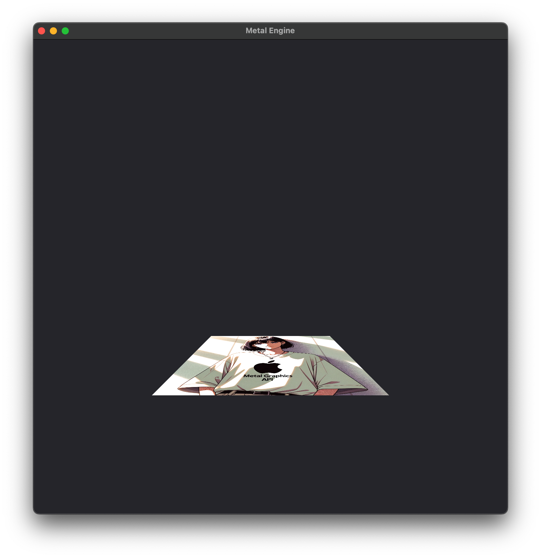
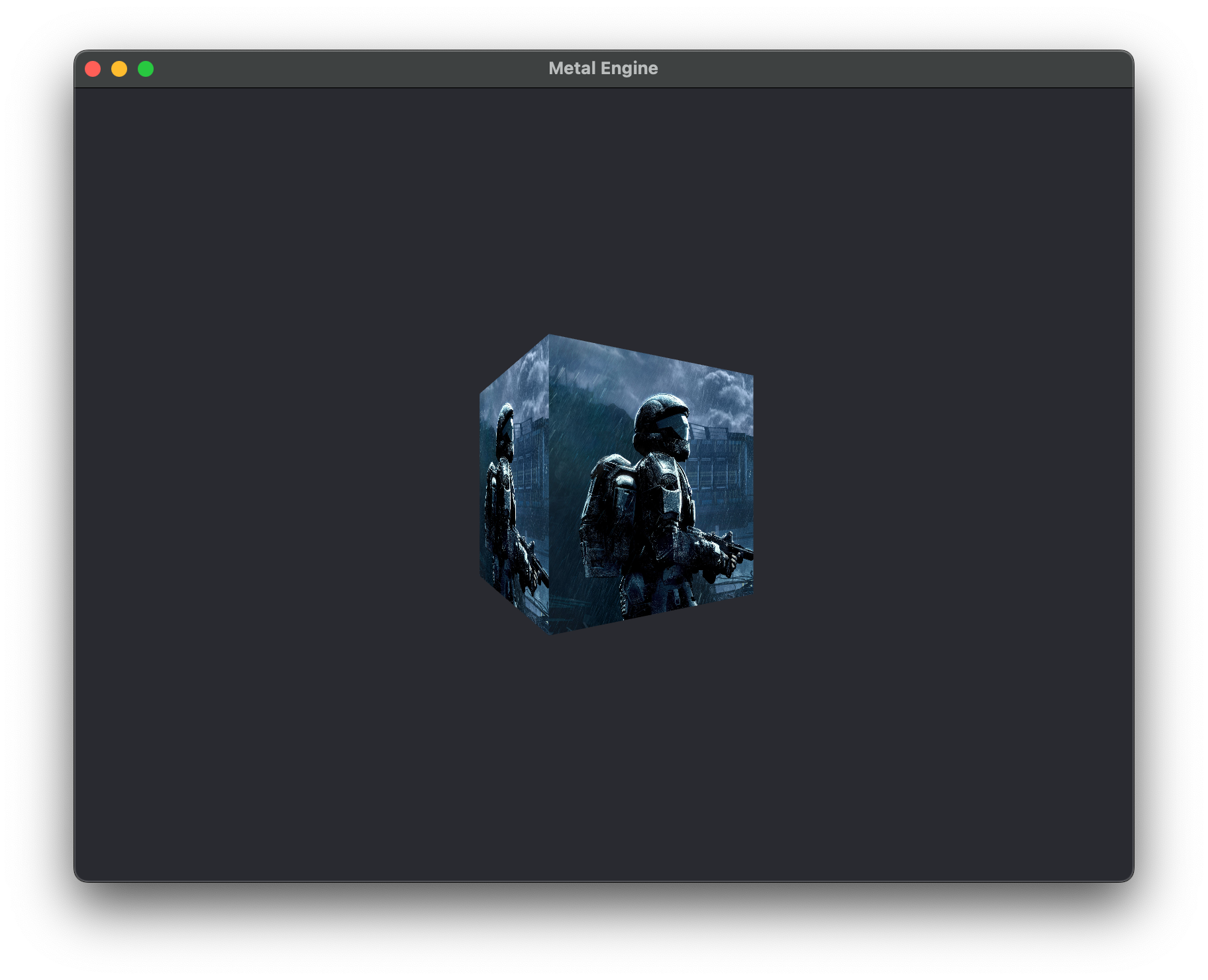
With this we can launch our application an- OH NO! What's this??
That doesn't look quite right does it? I've put a different texture on the cube to make the effect very obvious. One of the issues is that we don't have what's called a "depth buffer". The other issue is that all the faces of our cube are being rendered, because we haven't told Metal what winding order we're using or whether to cull the corresponding front or back faces. The winding order issue is an easy fix, but let's start to fix this mess by integrating a depth buffer into our renderer.
Setting up a Depth Buffer
A depth buffer, also known as a z-buffer, is an essential component in the land of computer graphics, particularly when rendering 3D scenes. Its primary purpose is to resolve visibility, i.e., to determine which objects (or parts of objects) are visible from a particular viewpoint and which are obscured by other objects. You should be able to understand this based on how our cube is rendering. The issue is, Metal is drawing the back face over the front face, which doesn't make any sense, but because we aren't using a depth buffer it doesn't know how to use the depth information to draw it correctly.
After Metal applies the viewport transformation to our objects in Normalized-Device Coordinate space, the coordinates of the objects are in screen space, which means they have specific pixel locations on the screen and depth values relative to the camera. When the rendering process begins, the depth buffer is created, essentially just as a texture that is same resolution as the rendering target (in our case, the screen), and each value in the depth buffer is typically set to a maximum, like 1.0 which corresponds to maximum z-depth in our Normalized-Device Coordinate space. In the standard rendering pipeline, after rasterization, fragments are processed in the fragment shader and then undergo depth testing.
After an individual fragment is processed by the fragment shader, the fragment undergoes depth testing, where the fragment's depth value is compared against the current value in the depth buffer for that fragments screen position. If the depth test passes, meaning the current fragment's z-value is lower than the current one, the depth buffer is updated with the fragment's depth value, and the fragment's color is then potentially written to the color buffer (after additional stages like blending). If however, the depth test fails, meaning that the depth value of the current fragment being processed is greater than the one in the depth buffer, the fragment is discarded, and its color isn't written into the color buffer.
You might think it strange or inefficient that the fragment shader might do all of that processing for an individual fragment, only to then perform the depth test and discard the fragment all together. In certain cases, you would certainly be right. This is why modern GPUs implement an optimization called early-z or early depth testing, where the GPU might actually check the depth of fragments before they're processed by the fragment shader. But, this can't be used in situations where the fragment shader modifies the depth value, or to give a more concrete example, when you're working with transparent objects like a glass window. While opaque objects can simply overwrite the color of a pixel if they're closer to the camera, transparent objects need to blend their color with whatever is already in the color buffer. As a result, transparent fragments can't simply discard fragments behind them, making Early-Z less effective.
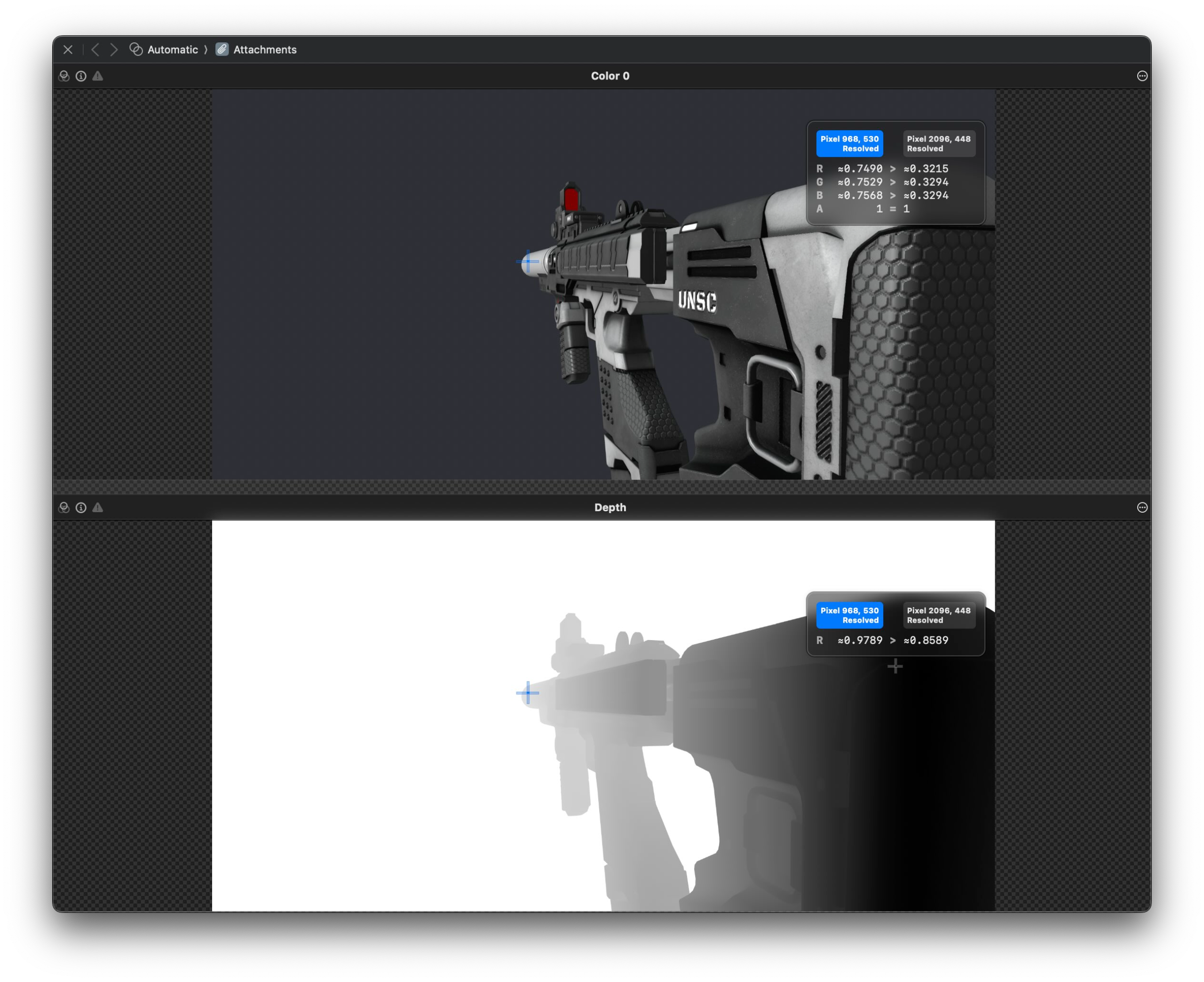
You can see in the image below what a depth buffer actually looks like compared to the final rendered image on the screen. The bottom image represents the depth buffer, where depth is based on what we call a "resolve" value or "R" value. An R value of 1.0 corresponds to an infinite distance, or the white background. The closer the objects gets to the camera, the darker the images becomes and the smaller the R value. If you look at the two points I've select on the 3D Model below for example, the point further away has a larger R value of 0.9789, compared to the point that's closer to the camera of 0.8589.
Multisample Anti-Aliasing
While we add our Depth Buffer, we're also going to implement Multisampled Anti-Aliasing (MSAA), which follows a very similar process to integrating our Depth Buffer into our renderer. MSAA is a technique used in computer graphics to improve image quality by reducing visual artifacts known as "aliasing". Aliasing occurs when the high-frequency details in an image can't be adequately represented at the resolution at which the image is sampled. This typically manifests as jagged edges or "jaggies" on objects in the image, especially along diagonal or curved lines. MSAA tries to solve this issue by sampling multiple color values within a single pixel and blending them together.
One benefit of MSAA is that it operates only on the edges of the geometry in our scene, making it more efficient than other techniques such as Super-Sampled Anti Aliasing (SSAA), which typically renders the entire scene at a 2-4x higher resolution and then downsamples the result. Additionally, MSAA invokes the fragment shader only once for each pixel, and shares the result among the samples. For testing whether a sample point is covered, the triangle depth is interpolated at each sample point that is covered and compared with the value in the depth buffer. The depth test is performed for each subsample, so its size must be adjusted based on the number of samples we'll be using per pixel. In our case, we're going to use 4 samples per pixel, so the depth buffer will be 4x the size as if we did not use MSAA at all.
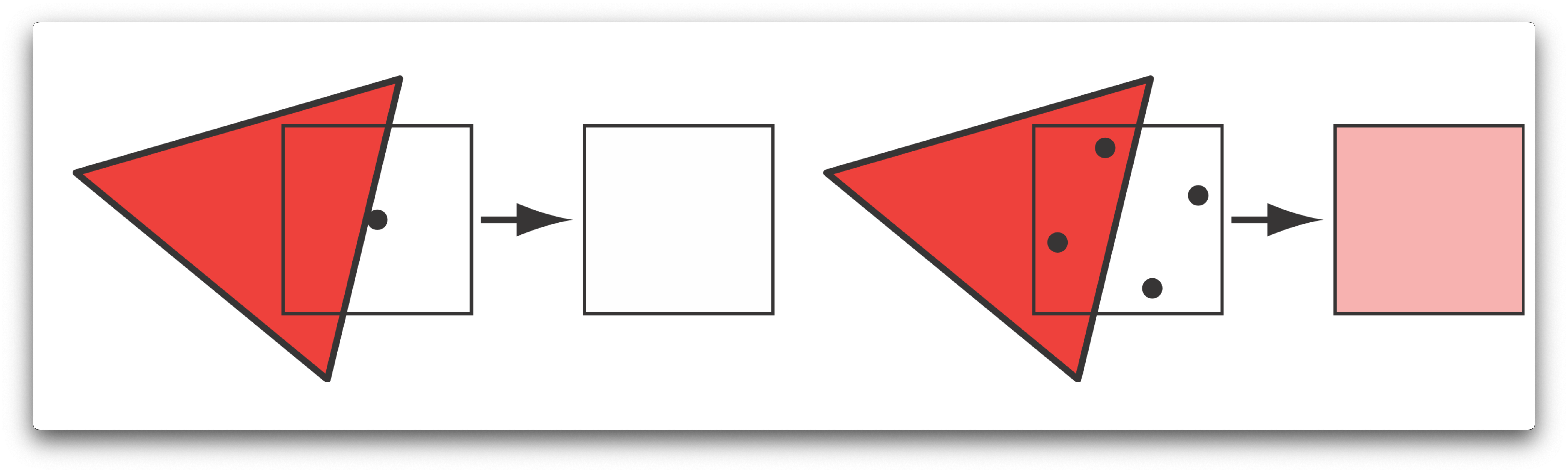
Take a look at the diagram below, on the left we have a triangle that overlaps part of a pixel on the screen. Without multi-sampling, the black dot in the center is used as the sampling point the rasterizer will use to pick the color that gets passed onto the fragment shader for that pixel. In this case, the triangle doesn't overlap with it so the final color is white. If you look at the example on the right however, we now have 4 sample points (hence, multisampling), two that lay in the triangle and two that lay outside of it. The rasterizer chooses one sample to pass on to the fragment shader to apply further processing. The final pixel color becomes a weighted blend of the colors of the 4 sampling points. In this case, since two samples lie inside the triangle, both of those samples will be assigned the color of the output of the pixel shader, and will be blended evenly with the color of the two samples laying outside of the triangle, giving us this final pinkish color.
This image is borrowed from Real Time Rendering, 3rd Edition.
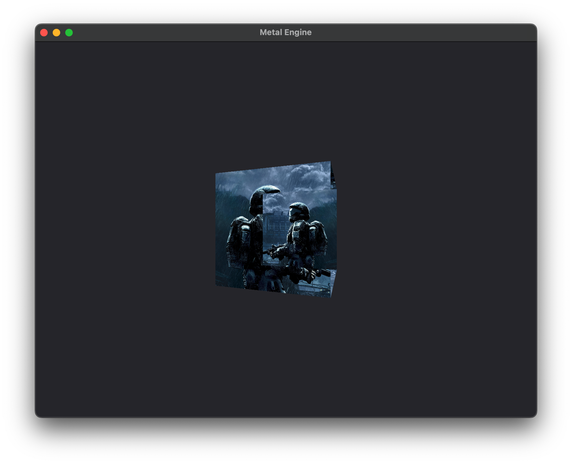
Below is a comparison of the edges of our cube, without MSAA, and with 4x MSAA enabled. You should notice that the image on the right has smoother edges than on the left.
| MSAA Disabled | 4x MSAA |
|---|---|
 |
 |
We're going to need to update our MTLEngine class by adding a view functions and member variables. In particular, we'll have a function createBuffers for allocating our transformation buffer on the GPU, and we'll need to create texture objects for our Depth Buffer and MSAA textures. We'll also abstract out our render pass descriptor creation to its own function, and have a function to recreate our Depth and MSAA textures when our window resizes. We're also going to create a variety of objects for holding our depth stencil state and depth/msaa textures, and abstracting out our renderpass descriptor:
class MTLEngine {
    ...
private:
    void createCube();
    void createBuffers();
    ...
    void createDepthAndMSAATextures();
    void createRenderPassDescriptor();

    // Upon resizing, update Depth and MSAA Textures.
    void updateRenderPassDescriptor();
    ...
    MTL::DepthStencilState* depthStencilState;
    MTL::RenderPassDescriptor* renderPassDescriptor;
    MTL::Texture* msaaRenderTargetTexture = nullptr;
    MTL::Texture* depthTexture;
    int sampleCount = 4;
}
We're adding quite a few things here. The first functions we'll update are our init() and cleanup() functions:
void MTLEngine::init() {
    initDevice();
    initWindow();

    createCube();
    createBuffers();
    createDefaultLibrary();
    createCommandQueue();
    createRenderPipeline();
    createDepthAndMSAATextures();
    createRenderPassDescriptor();
}
...
void MTLEngine::cleanup() {
    glfwTerminate();
    transformationBuffer->release();
    msaaRenderTargetTexture->release();
    depthTexture->release();
    renderPassDescriptor->release();
    metalDevice->release();
    delete grassTexture;
}
We'll first use our newly added createBuffers() function to create our transformation buffer. Make sure to remove the code we had in createCube() that created the transformation buffer earlier, and put it here:
void MTLEngine::createBuffers() {
    transformationBuffer = metalDevice->newBuffer(sizeof(TransformationData), MTL::ResourceStorageModeShared);
}
Before we create our MSAA and Depth Buffer Textures, we need to update our render pipeline creation:
void MTLEngine::createRenderPipeline() {
    MTL::Function* vertexShader = metalDefaultLibrary->newFunction(NS::String::string("vertexShader", NS::ASCIIStringEncoding));
    assert(vertexShader);
    MTL::Function* fragmentShader = metalDefaultLibrary->newFunction(NS::String::string("fragmentShader", NS::ASCIIStringEncoding));
    assert(fragmentShader);

    MTL::RenderPipelineDescriptor* renderPipelineDescriptor = MTL::RenderPipelineDescriptor::alloc()->init();
    renderPipelineDescriptor->setVertexFunction(vertexShader);
    renderPipelineDescriptor->setFragmentFunction(fragmentShader);
    assert(renderPipelineDescriptor);
    MTL::PixelFormat pixelFormat = (MTL::PixelFormat)metalLayer.pixelFormat;
    renderPipelineDescriptor->colorAttachments()->object(0)->setPixelFormat(pixelFormat);
    renderPipelineDescriptor->setSampleCount(sampleCount);
    renderPipelineDescriptor->setDepthAttachmentPixelFormat(MTL::PixelFormatDepth32Float);

    NS::Error* error;
    metalRenderPSO = metalDevice->newRenderPipelineState(renderPipelineDescriptor, &error);

    if (metalRenderPSO == nil) {
        std::cout << "Error creating render pipeline state: " << error << std::endl;
        std::exit(0);
    }

    MTL::DepthStencilDescriptor* depthStencilDescriptor = MTL::DepthStencilDescriptor::alloc()->init();
    depthStencilDescriptor->setDepthCompareFunction(MTL::CompareFunctionLessEqual);
    depthStencilDescriptor->setDepthWriteEnabled(true);
    depthStencilState = metalDevice->newDepthStencilState(depthStencilDescriptor);

    renderPipelineDescriptor->release();
    vertexShader->release();
    fragmentShader->release();
}
MTL::PixelFormatDepth32Float. We'll also add in some error handline for our PSO, , and create a depth stencil descriptor. We'll set our depth compare function to MTL::CompareFunctionLessEqual, so the depth test will pass if the current depth is closer or the same. We're also going to allow the gpu to write to the depth buffer, with setDepthWriteEnabled(true), since we're rendering only opaque objects here.
Next, we'll handle the creation of our MSAA and Depth Buffer Textures:
void MTLEngine::createDepthAndMSAATextures() {
    MTL::TextureDescriptor* msaaTextureDescriptor = MTL::TextureDescriptor::alloc()->init();
    msaaTextureDescriptor->setTextureType(MTL::TextureType2DMultisample);
    msaaTextureDescriptor->setPixelFormat(MTL::PixelFormatBGRA8Unorm);
    msaaTextureDescriptor->setWidth(metalLayer.drawableSize.width);
    msaaTextureDescriptor->setHeight(metalLayer.drawableSize.height);
    msaaTextureDescriptor->setSampleCount(sampleCount);
    msaaTextureDescriptor->setUsage(MTL::TextureUsageRenderTarget);

    msaaRenderTargetTexture = metalDevice->newTexture(msaaTextureDescriptor);

    MTL::TextureDescriptor* depthTextureDescriptor = MTL::TextureDescriptor::alloc()->init();
    depthTextureDescriptor->setTextureType(MTL::TextureType2DMultisample);
    depthTextureDescriptor->setPixelFormat(MTL::PixelFormatDepth32Float);
    depthTextureDescriptor->setWidth(metalLayer.drawableSize.width);
    depthTextureDescriptor->setHeight(metalLayer.drawableSize.height);
    depthTextureDescriptor->setUsage(MTL::TextureUsageRenderTarget);
    depthTextureDescriptor->setSampleCount(sampleCount);

    depthTexture = metalDevice->newTexture(depthTextureDescriptor);

    msaaTextureDescriptor->release();
    depthTextureDescriptor->release();
}
We first create our descriptors, and set various parameters such for each:
MSAA Texture
- Texture Type (TextureType2DMultisample): Specifies that this texture is a 2D texture with multiple samples per pixel, which is crucial for enabling MSAA.
- Pixel Format (PixelFormatBGRA8Unorm): Determines the format of the color data in the texture. BGRA8Unorm means it uses 8 bits for each of the blue, green, red, and alpha channels, and the data is normalized.
- Width and Height: These set the dimensions of the texture, usually matching the dimensions of the output framebuffer or drawable area.
- Sample Count: This is the number of samples per pixel and is a key setting for MSAA. More samples typically result in better anti-aliasing but at the cost of performance and memory usage. Here, we're using 4 samples.
- Usage (TextureUsageRenderTarget): Specifies how the texture will be used. Setting it as a render target means it can be written into by the GPU during rendering.
Depth Texture
- Texture Type (TextureType2DMultisample): Same as with the MSAA texture, specifies a 2D texture with multiple samples, which is necessary if you're using MSAA.
- Pixel Format (PixelFormatDepth32Float): Specifies that this texture will store depth information in a 32-bit floating-point format.
- Width and Height: Again, these usually match the dimensions of your framebuffer or drawable area.
- Usage (TextureUsageRenderTarget): Indicates that this texture will be used as a target for rendering operations, specifically for storing depth information.
- Sample Count: Must match the sample count of the MSAA texture for correct depth testing.
We'll also update our resizeFrameBuffer() and initWindow() functions:
void MTLEngine::resizeFrameBuffer(int width, int height) {
    metalLayer.drawableSize = CGSizeMake(width, height);
    // Deallocate the textures if they have been created
    if (msaaRenderTargetTexture) {
        msaaRenderTargetTexture->release();
        msaaRenderTargetTexture = nullptr;
    }
    if (depthTexture) {
        depthTexture->release();
        depthTexture = nullptr;
    }
    createDepthAndMSAATextures();
    metalDrawable = (__bridge CA::MetalDrawable*)[metalLayer nextDrawable];
    updateRenderPassDescriptor();
}

void MTLEngine::initWindow() {
    ...
    metalDrawable = (__bridge CA::MetalDrawable*)[metalLayer nextDrawable];
}
Additionally, note that at the end of our initWindow() function, we will actually need to first create a metalDrawable so that when we can properly create our MSAA/Drawable Textures for the first frame of our application.
Next, we'll implement our createRenderPassDescriptor() and updateRenderPassDescriptor() functions:
void MTLEngine::createRenderPassDescriptor() {
    renderPassDescriptor = MTL::RenderPassDescriptor::alloc()->init();

    MTL::RenderPassColorAttachmentDescriptor* colorAttachment = renderPassDescriptor->colorAttachments()->object(0);
    MTL::RenderPassDepthAttachmentDescriptor* depthAttachment = renderPassDescriptor->depthAttachment();

    colorAttachment->setTexture(msaaRenderTargetTexture);
    colorAttachment->setResolveTexture(metalDrawable->texture());
    colorAttachment->setLoadAction(MTL::LoadActionClear);
    colorAttachment->setClearColor(MTL::ClearColor(41.0f/255.0f, 42.0f/255.0f, 48.0f/255.0f, 1.0));
    colorAttachment->setStoreAction(MTL::StoreActionMultisampleResolve);

    depthAttachment->setTexture(depthTexture);
    depthAttachment->setLoadAction(MTL::LoadActionClear);
    depthAttachment->setStoreAction(MTL::StoreActionDontCare);
    depthAttachment->setClearDepth(1.0);
}

void MTLEngine::updateRenderPassDescriptor() {
    renderPassDescriptor->colorAttachments()->object(0)->setTexture(msaaRenderTargetTexture);
    renderPassDescriptor->colorAttachments()->object(0)->setResolveTexture(metalDrawable->texture());
    renderPassDescriptor->depthAttachment()->setTexture(depthTexture);
}
renderPassDescriptor creation out into it's own function, and creating it only once, whereas before we had its creation as part of our sendRenderCommand() function that was called every frame.
We'll create a color attachment which will serve as our msaaRenderTargetTexture, as well as a depth attachment for our depthTexture. We'll also create a function to update our renderPassDescriptor object every frame, by setting the msaaRenderTargetTexture and depthTexture, and we'll also set our resolve texture, our metalDrawable->texture(), which is the texture we want our MSAA sampling data to resolve to. In our case, the MSAA texture will have 4 samples per pixel, and it will blend these together into one pixel so that it can be stored in the metalDrawable texture, as the drawable is what's finally presented to the screen. Technically, we don't need to keep setting our MSAA and depth textures each frame, but I'm keeping it here anyways as the operation is basically free, and in the event that we resize our window, we can easily call this function to reset and resize these textures.
Next, we can update sendRenderCommand():
void MTLEngine::sendRenderCommand() {
    metalCommandBuffer = metalCommandQueue->commandBuffer();

    updateRenderPassDescriptor();
    MTL::RenderCommandEncoder* renderCommandEncoder = metalCommandBuffer->renderCommandEncoder(renderPassDescriptor);
    encodeRenderCommand(renderCommandEncoder);
    renderCommandEncoder->endEncoding();

    metalCommandBuffer->presentDrawable(metalDrawable);
    metalCommandBuffer->commit();
    metalCommandBuffer->waitUntilCompleted();
}
Here, we're simply having MTLEngine::sendRenderCommand() update our renderPassDescriptor object with the updateRenderPassDescriptor() function we just created , rather than recreating it every frame like we did previously.
void MTLEngine::encodeRenderCommand(MTL::RenderCommandEncoder* renderCommandEncoder) {
    matrix_float4x4 translationMatrix = matrix4x4_translation(0, 0.0, 0);

    float angleInDegrees = glfwGetTime()/2.0 * 90;
    float angleInRadians = angleInDegrees * M_PI / 180.0f;
    matrix_float4x4 rotationMatrix = matrix4x4_rotation(angleInRadians, 0.0, -1.0, 0.0);

    matrix_float4x4 modelMatrix = matrix_identity_float4x4;
    modelMatrix = simd_mul(translationMatrix, rotationMatrix);

    matrix_float4x4 viewMatrix = matrix4x4_translation(0.0, 0.0, 2.0);

    float aspectRatio = (metalLayer.frame.size.width / metalLayer.frame.size.height);
    float fov = 90 * (M_PI / 180.0f);
    float nearZ = 0.1f;
    float farZ = 100.0f;

    matrix_float4x4 perspectiveMatrix = matrix_perspective_left_hand(fov, aspectRatio, nearZ, farZ);
    TransformationData transformationData = { modelMatrix, viewMatrix, perspectiveMatrix };
    memcpy(transformationBuffer->contents(), &transformationData, sizeof(transformationData));

//    renderCommandEncoder->setTriangleFillMode(MTL::TriangleFillModeLines);
    renderCommandEncoder->setRenderPipelineState(metalRenderPSO);
    renderCommandEncoder->setDepthStencilState(depthStencilState);
    renderCommandEncoder->setVertexBuffer(cubeVertexBuffer, 0, 0);
    renderCommandEncoder->setVertexBuffer(transformationBuffer, 0, 1);
    MTL::PrimitiveType typeTriangle = MTL::PrimitiveTypeTriangle;
    NS::UInteger vertexStart = 0;
    NS::UInteger vertexCount = 36;
    renderCommandEncoder->setFragmentTexture(grassTexture->texture, 0);
    renderCommandEncoder->drawPrimitives(typeTriangle, vertexStart, vertexCount);
}
encodeRenderCommand() function, we are simply telling our renderCommandEncoder to set our Depth Stencil State that we created earlier, and voila, we should now have a 3D cube rendering with proper depth information taken into account and an image that has 4x MSAA applied.
Discarding Unecessary Faces and Fragments
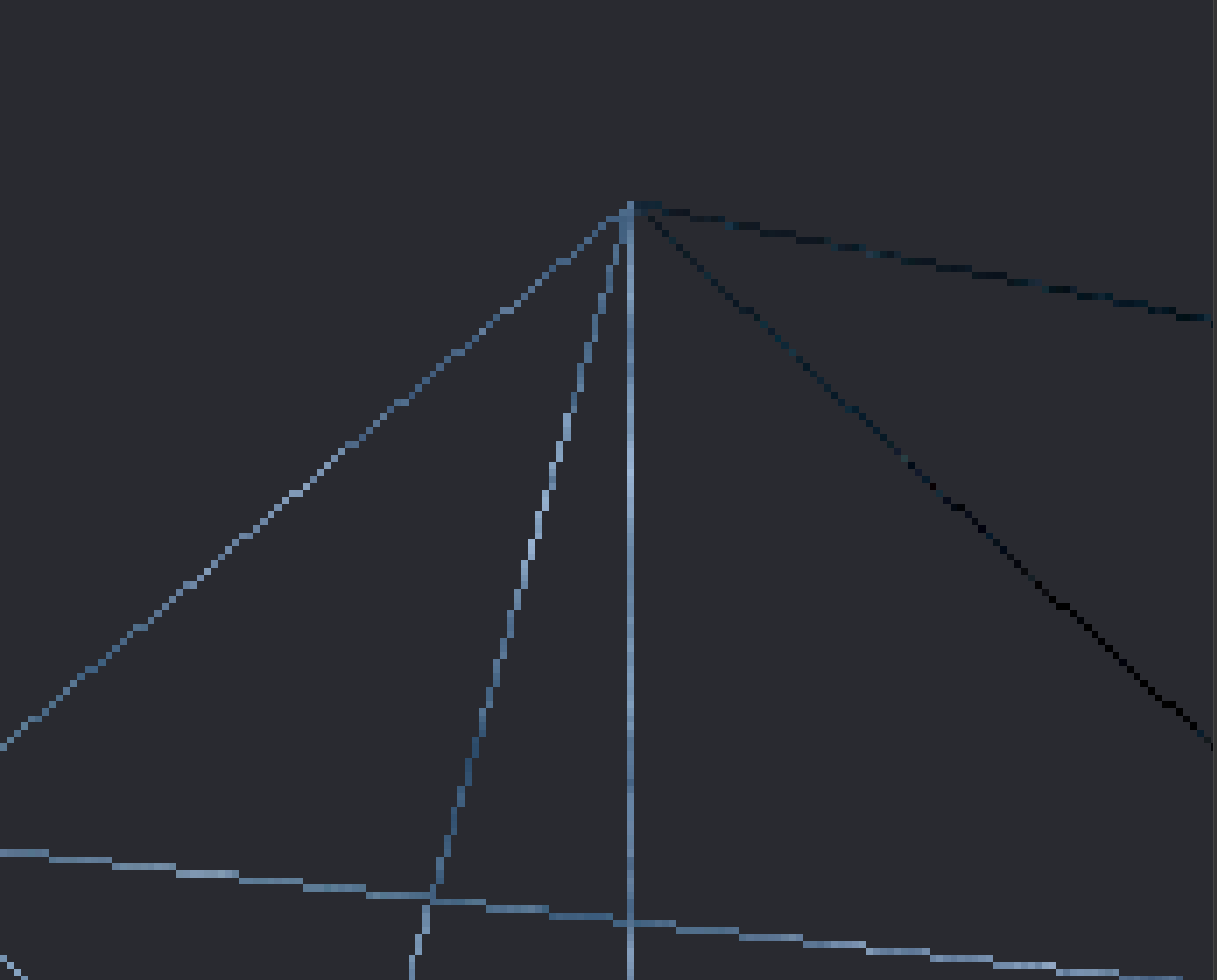
Even though we've implemented a depth buffer and MSAA into our renderer, we're still processing a lot of unecessary fragments. To demonstrate this, a look at the image below:
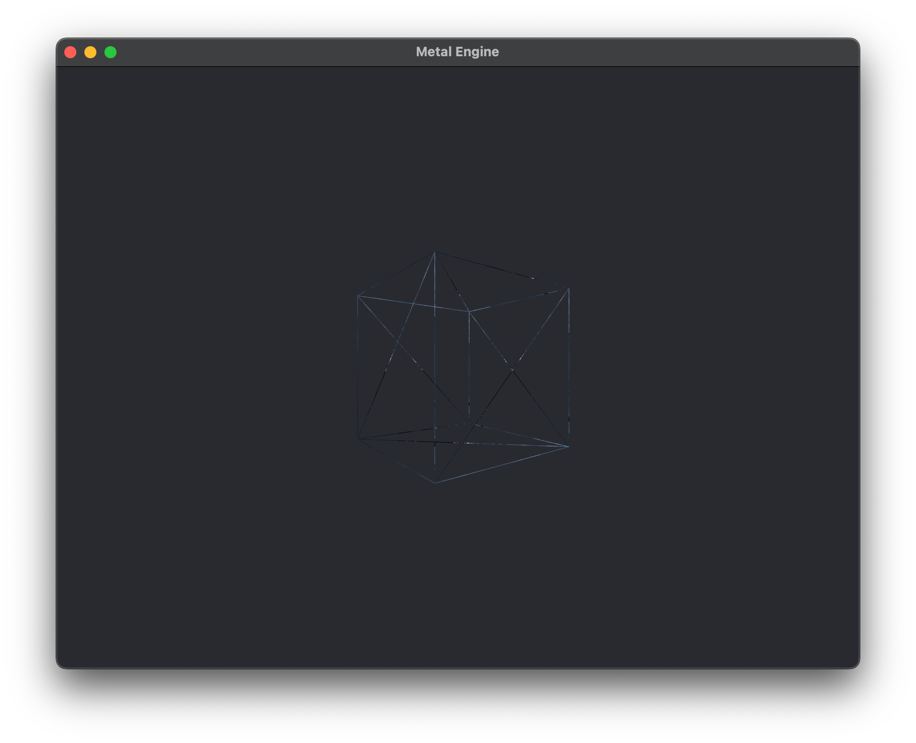
Remember how I said the rendering pipeline processes a fragment and then does does the depth test on it? When we render in wireframe mode, we can see that pretty clearly. We need to make sure we aren't processing all of those back faces and faces we can't see.
void MTLEngine::encodeRenderCommand(MTL::RenderCommandEncoder* renderCommandEncoder) {
...
    renderCommandEncoder->setFrontFacingWinding(MTL::WindingCounterClockwise);
    renderCommandEncoder->setCullMode(MTL::CullModeBack);
    renderCommandEncoder->setTriangleFillMode(MTL::TriangleFillModeLines);
    renderCommandEncoder->setRenderPipelineState(metalRenderPSO);
    renderCommandEncoder->setDepthStencilState(depthStencilState);
...
}
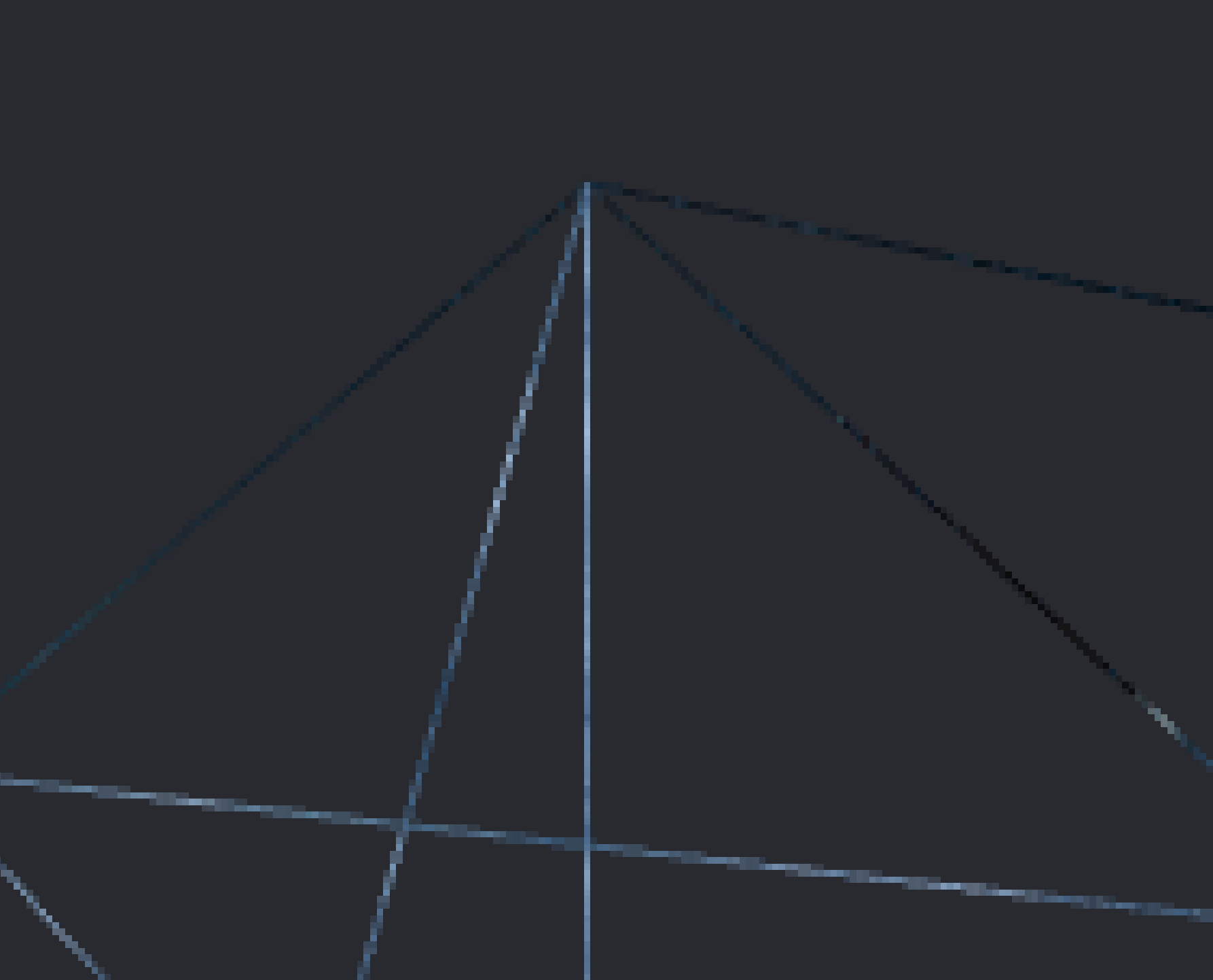
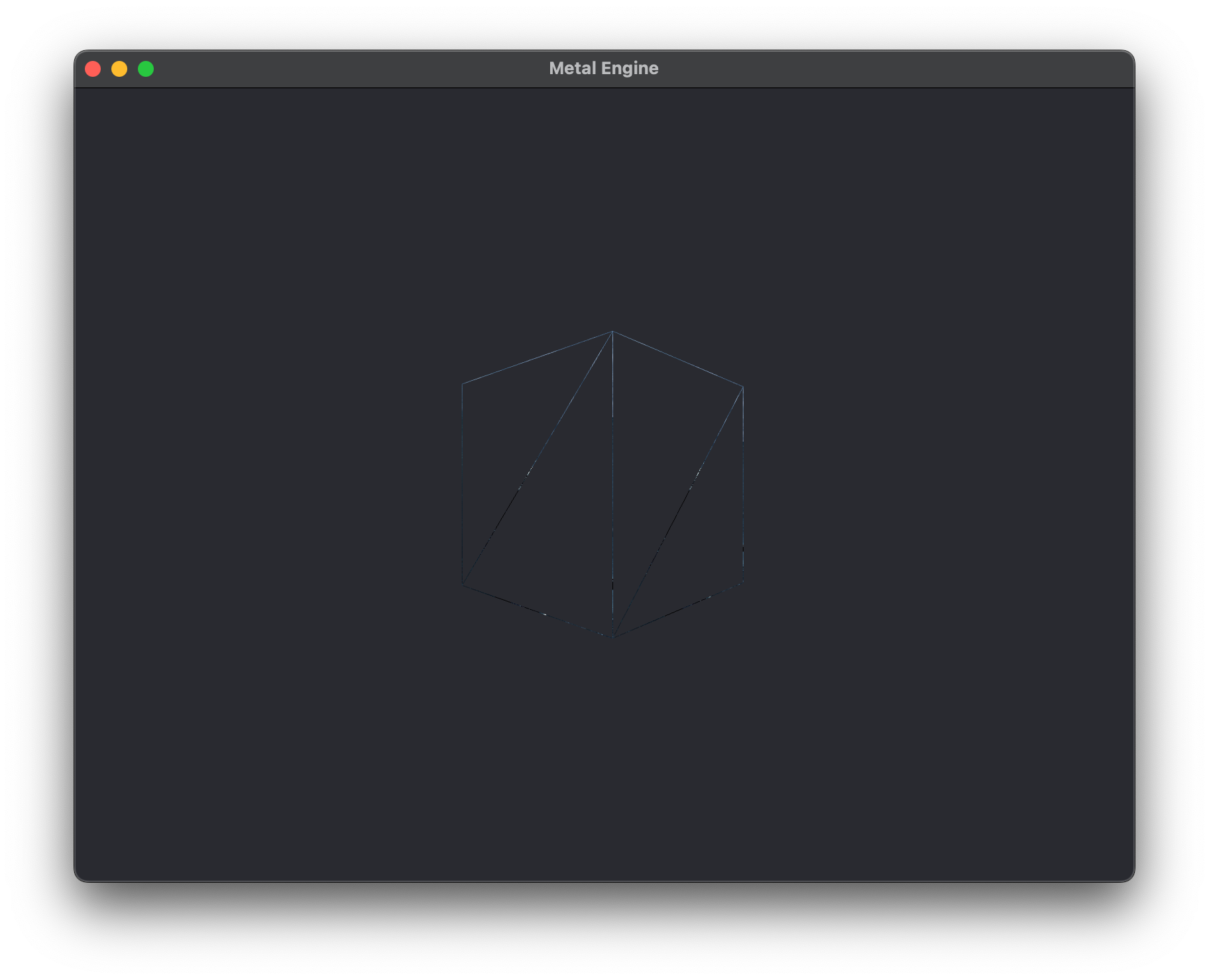
renderCommandEncoder to set the front face winding to MTL::WindingCounterClockwise, and to set the cull mode to MTL::CullModeBack so we can skip rendering those interior faces on the cube. Also notice here that I've set the triangle fill mode to MTL::TriangleFillModeLines so we can see the object in "wire-frame" mode. You can set it to MTL::TriangleFillModeFill to render like normal, or just leave it out and it will set that by default. And voila, we have a beautifully rendered wire-frame view of our cube, discarding the faces we can't see :D
The code for this chapter is accessible on the GitHub repository under branch Lesson_2_1.
-
This image references Figure 1 in Section 1.6 of the Metal Shading Language Specification 1.6 Metal Coordinate Systems. ↩